sftime2depth converts the input from vertical time to depth coordinates.

The following example from rsf/su/rsflab9 shows a seismic image converted from time to depth by this transformation:

The example is borrowed from John Stockwell’s lecture notes on Geophysical Image Processing and translated from Seismic Unix to Madagascar. The transformation follows the simple equation
$$t = 2\,\int\limits_{0}^{z} \frac{d\zeta}{v(\zeta)}$$,
where $t$ is two-way vertical time, $z$ is depth, and $v(z)$ is vertical velocity.

The sampling of the output depth axis is controlled by nz=, dz=, and z0=. If the velocity (provided in the auxiliary velocity= file) is sampled in time rather than depth, use intime=y. If it is slowness rather than velocity, use slow=y. If the input is in one-way time rather than two-way time, use twoway=n. The interpolation is carried out using B-splines. The spline order is controlled by extend=. By default, cubic splines (extend=4) are used.

The inverse transformation is given by sfdepth2time.

In the presence of lateral velocity variations, the correct transformation from time to depth is not as simple and needs additional corrections. See Time-to-depth conversion and seismic velocity estimation using time-migration velocity.

10 previous programs of the month

• sfwiggle
• sfvscan
• sfnmo
• sfpow
• sfpwd
• sfricker1
• sfhalfint
• sfbandpass
• sfkirmod
• sfiwarp

sfwiggle plots data using the traditional seismic method of wiggly traces.

The following example from rsf/rsf/rsftour shows a typical output:

Similarly to other plotting programs, there are multiple parameters that control the output. For example, poly=y draws solid polygons for highlighting positive data, transp=y transposes the two axes, xreverse=y or yreverse=y reverse the corresponding axis. Data scaling is controlled with either the absolute clip (clip=) or percentage clip (pclip=).

The following example uses transp=y poly=y yreverse=y pclip=100 unit2=km unit1=s label1=Time label2=Offset:

Use seemean=y to display lines corresponding to the mean value, use zplot= to control relative separation between different traces (the default is 0.75). The following example from bei/sg/toldi uses zplot=0.4:

Finally, sfwiggle makes it possible to plot irregularly sampled data by providing trace coordinates in xpos= file and (optionally) coordinate range with xmin= and xmax=. The following example from jsg/avo/avo2 shows a seismic gather displayed with (a) sfgrey in trace-number coordinates and (b) sfwiggle in offset coordinates.

10 previous programs of the month:

• sfvscan
• sfnmo
• sfpow
• sfpwd
• sfricker1
• sfhalfint
• sfbandpass
• sfkirmod
• sfiwarp
• sfpick

sfvscan implements seismic velocity analysis by scanning stacking velocities. This transformation is also known as the velocity transform or the hyperbolic Radon transform.

The following example from bei/vela/vscan shows an example for transforming a CMP (common midpoint) gather to a velocity (actually slowness) scan.

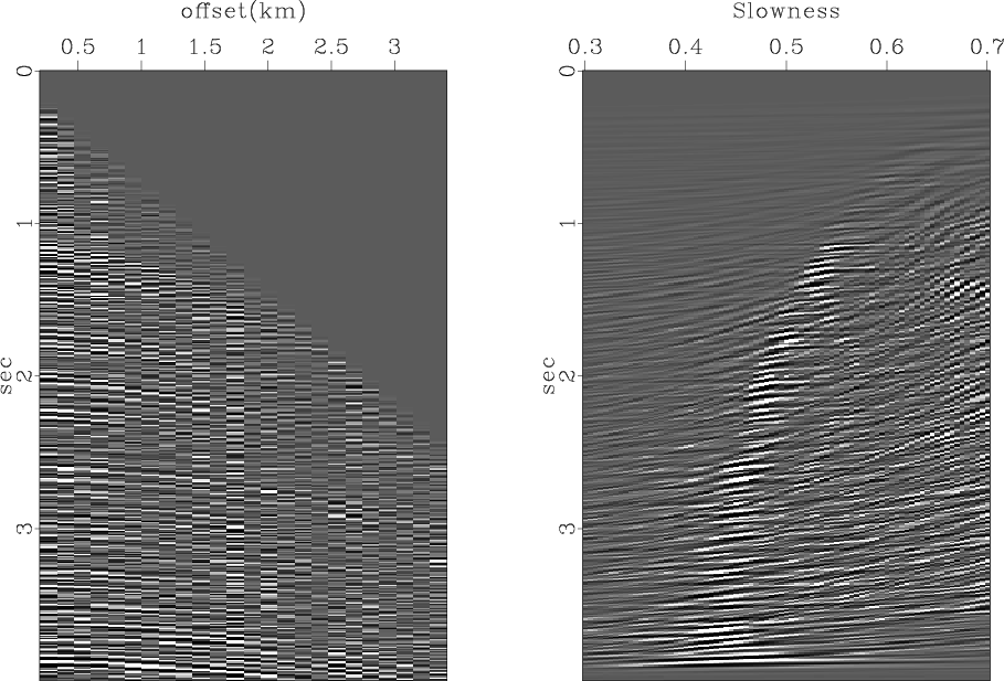
By default, sfvscan uses velocity as the horizontal axis. To change it to slowness, use slowness=y. It is also possible to use velocity or slowness squared by specifying squared=y. The range of velocities or slownesses to scan is given by v0=, dv=, nv=. In addition, it is possible to scan heterogeneity parameters in the shifted-hyperbola approximation using smax= and ns=.

The offset range in the input file is specified similarly to how it is done in sfnmo: The offset can be either regular (specified as the second axis in the input file) or irregular (specified in offset= file). By default, half-offset is used. To use full offset, specify half=n. Additionally, it is possible to specify a mask (with mask= file containing 1s and 0s) for skipping certain input traces during the scan.

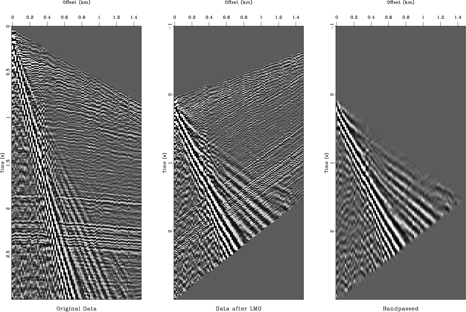
The NMO correction involved in velocity scanning is associated with the phenomenon of “NMO stretch”, a non-linear stretching of time at large offsets. The maximum allowed relative stretch is controlled by str= parameter. The part of the data that is stretched more than the allowed stretch gets muted. The width of the mute zone is controlled by mute= parameter.

By default, sfvscan outputs simple stack. To output semblance instead, use semblance=y or type=semblance. It is also possible to output other kinds of semblance attributes: differential semblance (type=w), AB semblance (type=a), or weighted semblance (type=w). See

Li, J., & Symes, W. W. (2007). Interval velocity estimation via NMO-based differential semblance. Geophysics, 72(6), U75-U88.

Sarkar, D., Castagna, J. P., & Lamb, W. J. (2001). AVO and velocity analysis. Geophysics, 66(4), 1284-1293.

Sarkar, D., Baumel, R. T., & Larner, K. L. (2002). Velocity analysis in the presence of amplitude variation. Geophysics, 67(5), 1664-1672.

Fomel, S. (2009). Velocity analysis using AB semblance. Geophysical Prospecting, 57(3), 311-321.

Luo, S., & Hale, D. (2012). Velocity analysis using weighted semblance. Geophysics, 77(2), U15-U22.

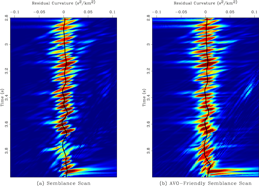
The following example from jsg/avo/avo2 shows a comparison between velocity scans computed using the conventional semblance and AB semblance.

For robustness, semblance values are averaged in time. The length of the averaging window in samples is given by nb= (the default is 2 time samples). By default, the input samples are stacked along the hyperbola with an asymptotically pseudounitary weight equal to the absolute value of offset times velocity. To apply a uniform weight, use weight=n. For the justification of the pseudounitary weighting, see

Claerbout, J. F., 1995, Basic Earth Imaging: Stanford Exploration Project.

S. Fomel, 2003, Asymptotic pseudounitary stacking operators: Geophysics, v. 68, 1032-1042.

For the operation inverse or adjoint to the velocity scan, use sfveltran, sfvelmod or sfvelinv.

For a faster implementation of the velocity scan (using the buttefly algorithm), use sfradon2.

From the output of the semblance scan computed with sfvscan, the velocity trend can be picked automatically with sfpick.

10 previous programs of the month

• sfnmo
• sfpow
• sfpwd
• sfricker1
• sfhalfint
• sfbandpass
• sfkirmod
• sfiwarp
• sfpick
• sffft3

sfzoom is a simple Tkinter script that allows for interactive zooming when viewing Vplot files generated by sfgrey. The zoomed images are created by windowing the original RSF file and therefore have the highest possible resolution.

Joe Dellinger has a more comprehensive plan for adding interactivity to Vplot graphics.

sfnmo implements normal moveout (NMO) correction, one of the most fundamental operations in seismic reflection data processing.

The following example from jsg/avo/avo shows synthetic data before and after NMO correction.

NMO transforms prestack seismic gathers by stretching each trace according to the equation
$$t = \sqrt{t_0^2 + \frac{x^2}{v^2(t_0)}}\;,$$
where $t$ is time before the correction, $t_0$ is time after the correction, $x$ is offset, and $v(t_0)$ is velocity specified in velocity= file. The NMO velocity can be picked (for example, with sfpick) from velocity scans (for example, produced with sfvscan).

If s= file is provided, sfnmo uses Malovichko’s shifted-hyperbola approximation
$$t \approx \left(1-\frac{1}{s(t_0)}\right) + \frac{1}{s(t_0)}\,\sqrt{t_0^2 + s(t_0)\,\frac{x^2}{v^2(t_0)}}$$
See

• Malovichko, A. A., 1978, A new representation of the traveltime curve of reflected waves in horizontally layered media: Applied Geophysics (in Russian), 91, 47-53
• Sword, C. H., 1987, A Soviet look at datum shift, in SEP-51: Stanford Exploration Project, 313-316.
• de Bazelaire, E., 1988, Normal moveout revisited – Inhomogeneous media and curved interfaces: Geophysics, 53, 143-157.
• Castle, R. J., 1994, Theory of normal moveout: Geophysics, 59, 983-999.

If a= file is provided, sfnmo uses Taner’s velocity-acceleration approximation
$$t = \sqrt{t_0^2 + \frac{x^2}{v^2(t_0)+a(t_0)\,x^2}}$$
See

• Taner, M. T., S. Treitel, and M. Al-Chalabi, 2005, A new travel time estimation method for horizontal strata: 75th Ann. Internat. Mtg, Soc. of Expl. Geophys., 2273-2276.
• Taner, M. T., S. Treitel, M. Al-Chalabi, and S. Fomel, 2007, An offset dependent NMO velocity model: EAGE 69th Conference and Exhibition, EAGE, P036.

The offset $x$ can be either regular (specified as the second axis in the input file) or irregular (specified in offset= file). By default, half-offset is used $h=x/2$. To use full offset, specify half=n.

Additionally, it is possible to specify a mask (with mask= file containing 1s and 0s) for skipping certain traces during the correction. See the following example from rsf/scons/rsf

The NMO correction is associated with the phenomenon of “NMO stretch”, a non-linear stretching of time at large offsets. The maximum allowed relative stretch is controlled by str= parameter. The part of the data that is stretched more than the allowed stretch gets muted. The width of the mute zone is controlled by mute= parameter.

NMO with constant velocity can be accomplished with sfnmostretch. For 3-D azimuthally-anisotropic moveout correction, try sfnmo3. For NMO in the tau-p domain, try sftaupmo. For an inverse NMO operation, try sfnimo.

10 previous programs of the month

• sfpow
• sfpwd
• sfricker1
• sfhalfint
• sfbandpass
• sfkirmod
• sfiwarp
• sfpick
• sffft3
• sfdip

sfpow multiplies the input data by a gain function of the form
$$G(x_1,x_2,\ldots,x_n)=x_1^{p_1}\,x_2^{p_2} \cdots x_n^{p_n}$$
The powers $p_1,p_2,\ldots,p_n$ are given by pow1=, pow2=, etc. parameters.

For backward compatibility, sftpow tpow= is an alias for sfpow pow1=.

The following example from geo391/hw1/tpow shows an application of sfpow pow1=2 *to a shot gather. The gain of *pow1=2 for seismic data was advocated by Jon Claerbout.

To estimate an appropriate power gain from the data, you can try sffpow.

10 previous programs of the month

• sfpwd
• sfricker1
• sfhalfint
• sfbandpass
• sfkirmod
• sfiwarp
• sfpick
• sffft3
• sfdip
• sfderiv

sfpwd implements plane-wave destruction, a filter that attenuates locally plane-wave events, as described in the paper Applications of plane-wave destruction filters.

The following example from jsg/diffr/gom shows a seismic section before and after an application of sfpwd:

sfpwd takes two input files: a 2-D or 3-D seismic data, and the local slope estimated by sfdip and specified by dip= parameter. When applied to 3-D data, sfpwd can produce either one output (inline or crossline destruction) or two outputs (both inline and crossline desctructions). This is controlled by the which= parameter. Other parameters (nj1=, nj2=, order=) have the same meaning as the corresponding parameters in sfdip.

10 previous programs of the month:

• sfricker1
• sfhalfint
• sfbandpass
• sfkirmod
• sfiwarp
• sfpick
• sffft3
• sfdip
• sfderiv
• sfgrey3

sfricker1 implements 1-D convolution with the Ricker wavelet.

The following example from rsf/rsf/wedge shows convolution modeling with a wedge model using sfricker1.

The convolution is implemented in the frequency domain, where the Ricker wavelet takes the form
$$F(\omega) = \frac{\omega^2}{\omega_0^2}\,\exp\left(-\frac{\omega^2}{\omega_0^2}\right)$$
The peak frequency $\omega_0$ can be specified either in hertz (with frequency= parameter) as a fraction of the Nyquist frequency (with freq= parameter). Optionally, it is possible to combine the Ricker wavelet with a half-order derivative filter using deriv=y.

10 previous programs of the month

• sfhalfint
• sfbandpass
• sfkirmod
• sfiwarp
• sfpick
• sffft3
• sfdip
• sfderiv
• sfgrey3
• sfspectra

sfhalfint implements half-order integration or differentiation, a filtering operation common in 2-D imaging operators such as as slant stacking or Kirchhoff migration.

By default, sfhalfint performs half-order integration. To apply half-order differentiation, use inv=y. To apply the adjoint operator, use adj=y.

Theoretically, half-order integration and differiation correspond to division by $(i\omega)^{1/2}$. For stability, $i\omega$ is replaced in practice by $1-\rho\,Z$ when doing differentiation and by $\frac{1}{2}\,\frac{1-\rho\,Z}{1+\rho\,Z}$ when doing integration. Here $Z=e^{i\omega\,\Delta t}$. As explained by Jon Claerbout, this approximation attenuates high frequencies and assures a causal impulse response. The value of the $\rho$ parameter is controlled by rho=.

The following plot from bei/ft1/hankel shows the impulse response of half-order differentiation (also known as the “rho filter”)

10 previous programs of the month

• sfbandpass
• sfkirmod
• sfiwarp
• sfpick
• sffft3
• sfdip
• sfderiv
• sfgrey3
• sfspectra
• sfnoise

sfbandpass implements bandpass filtering using the Butterworth algorithm.

The desired bandwidth is specified by low and high frequencies (in Hertz) flo= and fhi=. A continuous low-pass Butterworth filter is given by
$$B_N^2(\omega) = \displaystyle \frac{1}{\displaystyle 1+\left(\frac{\omega}{\omega_0}\right)^{2N}}$$
The actual filtering is implemented by recursive (Infinite Impulse Response) convolution in the time domain. The number of poles ($N$) for the low-pass and high-pass filters are specified by nplo= and nphi= parameters.

The following example from sep/pwd/hector shows a land shot gather after linear moveout and low-pass filtering that isolates ground-roll noise.

By default, the applied filter has zero phase. To use a minimum-phase filter, use phase=y. This is the option used in the Madagascar test example from rsf/rsf/test

An alternative way to implement bandpass filtering is using the Fourier transform and tapering functions in the Fourier domain. One example of this approach is provided by sferf.

10 previous programs of the month

• sfkirmod
• sfiwarp
• sfpick
• sffft3
• sfdip
• sfderiv
• sfgrey3
• sfspectra
• sfnoise
• sfgraph