sfdip estimates a local slope (dip) using the plane-wave destruction algorithm.
The dip is measured in time samples. If $\alpha$ is the dip angle, then the output of sfdip corresponds to the dimensionless quantity $p=\tan{\alpha}$.
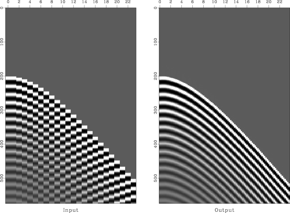
The following example from jsg/flat/flat shows an input synthetic dataset and an estimated dip field


When applied to 3-D data, sfdip outputs a 4-D file with n4=2 and two dips (inline and crossline). To compute only the inline dip, use n4=0. To compute only the crossline dip, use n4=1. The following example from sep/plane/qint shows an input synthetic 3-D dataset and the two dip components calculated from it.


The algorithm consists of a number of non-linear Gauss-Newton iterations (specified by niter=) with a number of linear CG-shaping iterations (specified by liter=) inside each non-linear cycle. The convergence depends on the initial dip values, which can be specified either as constants (p0= and q0=) or as auxiliary input files (idip= and xdip=). If it is necessary to constrain the range of dip values, it can be controlled by specifying minimum or maximum parameters (pmin=, pmax= and qmin=, qmax=). The smoothness of the dip is assured by shaping regularization and controled by the smoothing radii rect1=, rect2=, rect3=.
With default parameters, the dip estimate is accurate only up to 45 degrees. To estimate steeper (aliased) dips, increase the order= parameter. The order of the filter corresponds to the maximum dip. Alternatively, one can use the technique of filter stretching (interlacing), explained by Claerbout; the stretching parameters are nj1= and nj2=. The following examples from sep/pwd/alias show aliased data interpolation using (a) order=12 (b) order=3 nj1=4.

For a faster version, with only one non-linear iteration but with fewer options, try sffdip. To estimate two interfering dips, try sftwodip2. To estimate a number of constant dips, try sfdips.
codemore code
~~~~