Waves and Fourier sums

Hankel tail

The waveform in equation (31) often arises in practice (as the 2-D Huygens wavelet). Because of the discontinuities on the left side of equation (31), it is not easy to visualize. Thinking again of the time derivative as a convolution with the doublet $(1,-1)/\Delta t$, we imagine the 2-D Huygen's wavelet as a positive impulse followed by negative signal decaying as $-t^{-3/2}$. This decaying signal is sometimes called the ``Hankel tail.'' In the frequency domain $-i\omega= \vert\omega \vert e ^ {-i90^\circ}$ has a 90 degree phase angle and $\sqrt{-i\omega}= \vert\omega \vert^{1/2} e ^ {-i45^\circ}$ has a 45 degree phase angle.

api/c/halfint.c

    for (i=0; i < nw; i++) {
	om = -2.*SF_PI*i/n;
	cw.r = cosf(om);
	cw.i = sinf(om);

	cz.r = 1.-rho*cw.r;
	cz.i = -rho*cw.i;
	if (inv) {
	    cz = sf_csqrtf(cz);
	} else {
	    cz2.r = 0.5*(1.+rho*cw.r);
	    cz2.i = 0.5*rho*cw.i;
	    cz = sf_csqrtf(sf_cdiv(cz2,cz));
	}
	cf[i].r = cz.r/n;
	cf[i].i = cz.i/n;
    }

In practice, it is easiest to represent and to apply the 2-D Huygen's wavelet in the frequency domain. Subroutine halfint() is provided for that purpose. Instead of using $\sqrt{-i\omega}$ which has a discontinuity at the Nyquist frequency and a noncausal time function, I use the square root of a causal representation of a finite difference, i.e. $\sqrt{1-Z}$, which is well behaved at the Nyquist frequency and has the advantage that the modeling operator is causal (vanishes when $t<t_0$). 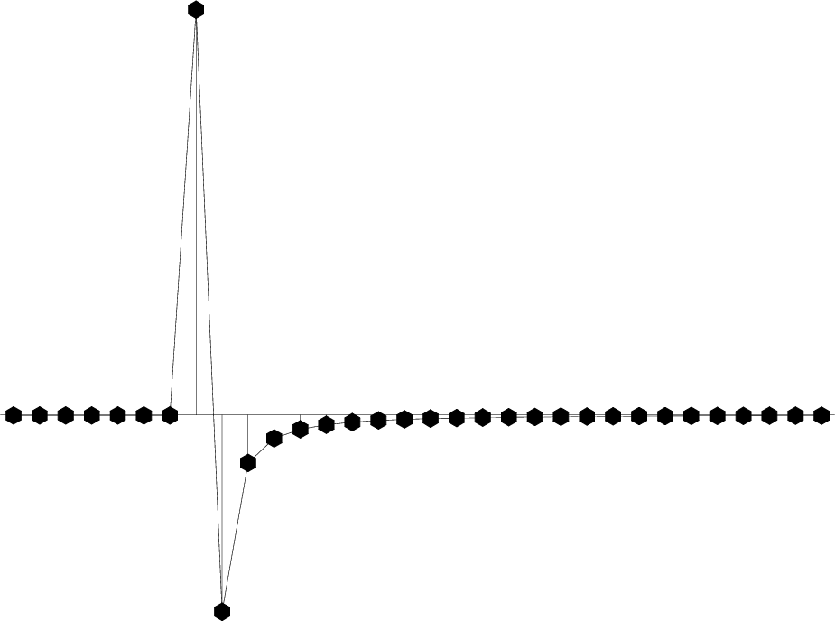Passing an impulse function into subroutine halfint() gives the response seen in Figure 9.

hankel Figure 9. Impulse response (delayed) of finite difference operator of half order. Twice applying this filter is equivalent to once applying $(1,-1)$.

Waves and Fourier sums