sfmig2 implements 2-D prestack Kirchhoff time migration.

The program is using triangle antialiasing filters.

J. F. Claerbout, 1992, Anti Aliasing: SEP-73, Stanford Exploration Project, 371-390.

D. E. Lumley, J. F. Claerbout, and D. Bevc, 1994, Anti-aliased Kirchhoff 3-D migration: SEG Annual Meeting, Expanded Abstracts, 1282-1285.

The following example from sep/aal/gulf shows migration applied to a near-offset section from the Gulf of Mexico.

The amount of antialiasing is controlled by antialias= parameter.

A half-derivative waveform-correction filter (rho filter) is applied and is controlled by rho= parameter.

The program has an adjoint flag adj= and can be used as a linear operator. The default value adj=y corresponds to migration, adj=n corresponds to modeling (demigration).

An additional required input is vel= (time-migration velocity). An optional output is gather= (common-offset image gathers).

10 previous programs of the month:

• sfsort
• sfdivn
• sfpldb and sfplas
• sfisolr2
• sfsimilarity
• sfmutter
• sfintbin
• sfbox
• sfslant
• sfgrey

sfsort sorts the input by absolute value.

It takes either floating-point or complex input. Here is a quick example:

bash$ sfspike n1=10 | sfnoise rep=y seed=2016 > random.rsf
bash$ < random.rsf sfdisfil
   0:       -0.3485      -0.3108       0.7928      0.01292      -0.5301
   5:       -0.4556      -0.2901      -0.7167       -1.209      -0.2871
bash$  < random.rsf sfsort | sfdisfil
   0:         1.209       0.7928       0.7167       0.5301       0.4556
   5:        0.3485       0.3108       0.2901       0.2871      0.01292

To sort in reverse (ascending) order, use ascmode=y:

 
bash$ < random.rsf sfsort ascmode=y | sfdisfil
   0:       0.01292       0.2871       0.2901       0.3108       0.3485
   5:        0.4556       0.5301       0.7167       0.7928        1.209

sfsort tries to perform sorting in memory but, if the input is too large, it switches to slower out-of-core operations. To control the amount of available memory, use memsize= parameter.

If the input is multidimensional, and you want to sort data only up to a certain dimension, use dim= parameter. In the following example, each of the two rows is sorted independently:

bash$ < random.rsf sfput n1=5 n2=2 | sfsort dim=1 | sfdisfil
   0:        0.7928       0.5301       0.3485       0.3108      0.01292
   5:         1.209       0.7167       0.4556       0.2901       0.2871

sfsort was contributed to Madagascar by Gilles Hennenfent and Henryk Modzelewski from SLIM, UBC. They provide the following test example in slim/slimUserManual/sfsort:

10 previous programs of the month:

• sfdivn
• sfpldb and sfplas
• sfisolr2
• sfsimilarity
• sfmutter
• sfintbin
• sfbox
• sfslant
• sfgrey
• sfhistogram

sfdivn divides two signals, producing a smooth output. It treats division as inversion and regularizes the inversion using shaping regularization.

The following example from jlu/riesz/sigmoid shows the local dip computed by a smooth division of two components of the Riesz transform.

The denominator file is provided by den=. The shaping regularization is controlled by smoothness radii rect1=, rect2=, etc. and the maximum number of iterations niter=. The iterations can be accelerated by using eps= parameter. To suppress the output of iteration statistics on the screen, use verb=n.

10 previous programs of the month:

• sfpldb and sfplas
• sfisolr2
• sfsimilarity
• sfmutter
• sfintbin
• sfbox
• sfslant
• sfgrey
• sfhistogram
• sfmf

sfpldb and splas are utilities for debugging Vplot files by converting them to the plain text (ASCII) form. pldb (plot debugger) converts a Vplot file to a text form, plas (plot assembler) converts the text form back to the Vplot format.

Suppose, for example, that your Vplot file has a typo in the label which spells Dept instead of Depth. Here is a Unix one-liner for fixing the label:

< file.vpl sfpldb | sed s/Dept/Depth/ | sfplas > fixed.vpl

Here the Unix line editor sed gets sandwiched between sfpldb and sfplas.

These programs were initinally developed by Vplot’s original author, Joe Dellinger.

10 previous programs of the month:

• sfisolr2
• sfsimilarity
• sfmutter
• sfintbin
• sfbox
• sfslant
• sfgrey
• sfhistogram
• sfmf
• sfbin

sfwxipick is a new interactive picking script which reimplements the functionality of sfipick using wxpython.

See also sfwxzoom which reimplements the functionality of sfzoom. These functionalities can be easily extended if needed. Enjoy!

• Is there a Graphical User Interface to Madagascar?
• How do I do interactive picking?
• Zooming in Vplot

sfisolr2 performs low-rank decomposition for wave propagation in a 2-D isotropic medium using lowrank approximation method.

The output of sfisolr2 can be used by other programs, such as sffftwave2 or sffftexp0 to perform wave modeling or reverse-time migration.

The following example from tccs/lowrank/impres shows a wave snapshot from a point source in an isotropic medium with a variable velocity.

sfisolr2 takes two inputs: the velocity model as standard input and the file given by fft= to specify the dimensions of the Fourier-transformed grid (the values in this file are not used). The program produces two outputs: the right decomposition matrix in the standard output, and the left decomposion matrix specified by left=. To make the results reproducible despite the randomization algorithm, set seed= for pseudorandom number generation.

The rank of the lowrank approximation is controlled by several parameters. The most important of those is the time step size dt=. The other controlling parameters are the approximation tolerance eps= and the number of random probes (maximum rank) npk=.

The related programs are sfanisolr2 for the anisotropic (TTI) case, and sfisolr3 for the 3-D case. The following example from tccs/lowrank/threed shows a 3-D wavefield snapshot computed with sfisolr3:

10 previous programs of the month:

• sfsimilarity
• sfmutter
• sfintbin
• sfbox
• sfslant
• sfgrey
• sfhistogram
• sfmf
• sfbin
• sfthreshold

sfsimilarity computes the local similarity attribute between two datasets.

The following example from tccs/ortho/orthofair shows two 2-D sections and their local similarity.

The second dataset for computing the local similarity is specified by other=. The program performs iterations of shaping regularization. The main controling parameters are the number of iterations niter= and the smoothing radii in different dimensions rect1=, rect2=, etc. The iterations can be additionally accelerated using the eps= parameters. To suppress the output of iteration statistics on the screen, use verb=n.

10 previous programs of the month:

• sfmutter
• sfintbin
• sfbox
• sfslant
• sfgrey
• sfhistogram
• sfmf
• sfbin
• sfthreshold
• sfsigmoid

sfslant is a T-X implementation of slant stack, also known as Radon transform or tau-p transform.

The two middle panels in the example below from cwp/geo2006TimeShiftImagingCondition/zicig show a time-shift common-image gather and its transformation by slant stack.

sfslant is a linear operator and has an adjoint flag adj=: When adj=n, the transformation is from tau-p to t-x. When adj=y, the transformation is from t-x to tau-p. The sampling on the transformed coordinate is controlled in the two cases by nx=, dx=, x0= or, respectively np=, dp=, p0=. Antialiasing is enabled by default with anti=1 parameter. The central slope for antialiasing is given by p1=. A space integration is sfslant generally requires a corrective “rho filter” (half-order differentiation). It is enabled by rho= parameter.

For an F-X implementation of the Radon transform, see sfradon.

10 previous programs of the month

• sfgrey
• sfhistogram
• sfmf
• sfbin
• sfthreshold
• sfsigmoid
• sfmax1
• sfstolt
• sfltft
• sfeikonal

There are many different libraries for GUI (graphical user interfaces), many of them with Python bindings: PyGTK, PyQt, PySide, etc. Tkinter is one of the oldest Python GUI libraries and is considered to be the standard one. Another popular choice is wxPython, a Python interface for wxWidgets C++ library.

A quick example of wxPython is provided in wxvpconvert, a silly GUI for Madagascar’s vpconvert script. Compare with tkvpconvert.

See also:

• Is there a Graphical User Interface to Madagascar?
• Madagascar in the cloud
• Tutorial on parameter testing

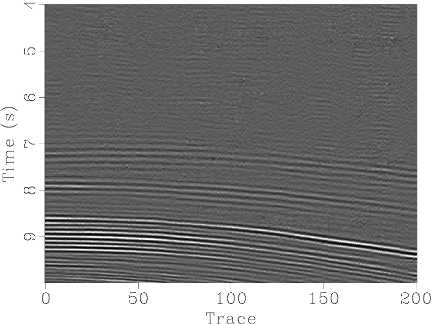
sfgrey is the most widely used program in Madagascar. It is used for plotting multidimensional images with grayscale or pseudocolor.

sfgrey shares many of its options with other plotting programs, such as sfgraph, sfwiggle, and sfcontour. You can look for common options by running sfdoc stdplot or checking out stdplot documentation online.

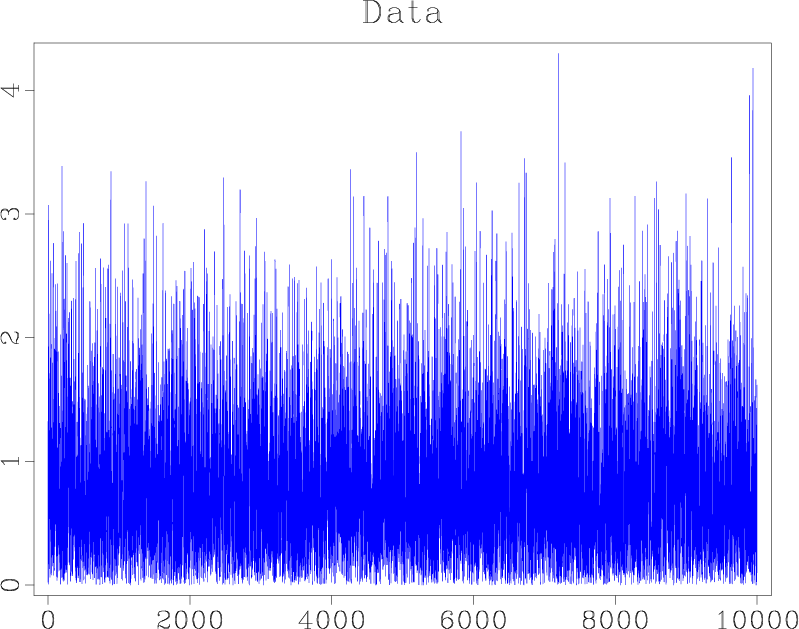
Parameters that control the range of data to be displayed are clip=, pclip=, bias=, allpos=, mean=. The default behavior is pclip=99, which means that data values get clipped to the 99-nth percentile. To display values without clipping, use pclip=100. Setting the clip value with clip= takes the precedence over setting the percentage clip with pclip=. The bias= defines the data value for the middle of the color scale range, the default (appropriate for seismic data) is bias=0. When displaying values that are all larger than the bias value, set allpos=y (all positive). To set the bias to the mean value of the data without specifying it explicitly, use mean=y. The following example from trip/asg/project uses mean=y to display a synthetic model.

The gpow= parameter applies a nonlinear scaling by taking the image to the corresponding power. If the value of gpow is less than zero, the appropriate value is estimated from the data. The following example from gee/pch/ida uses the value of gpow=0.25.

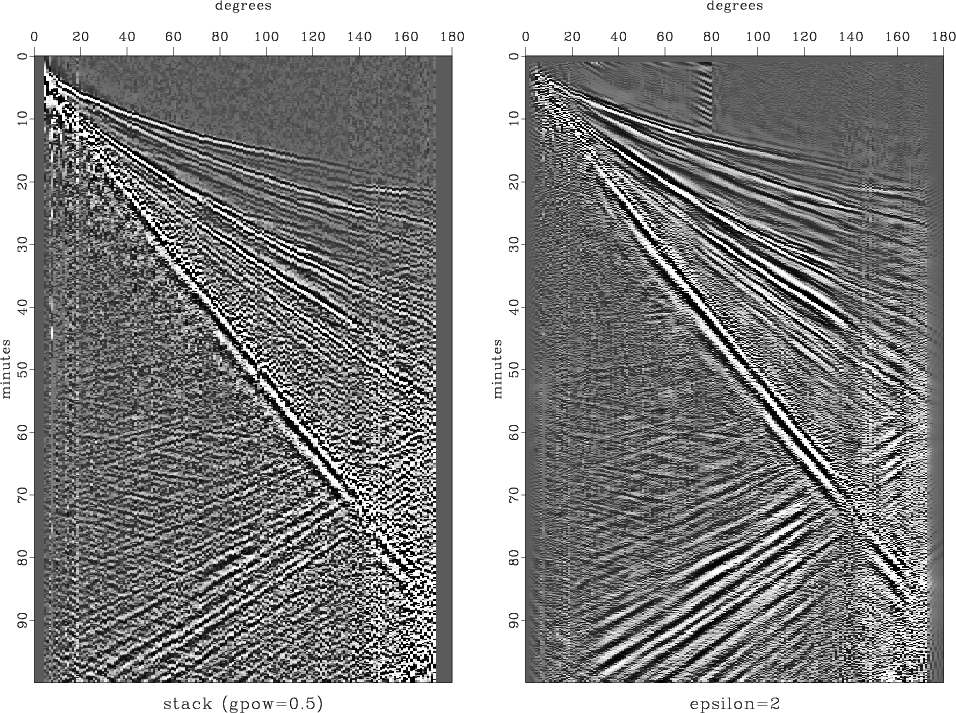
If the input is a 3-D cube, sfgrey can use a particular panel (2-D slice) to estimate clip or glow. The panel is specified by gainpanel= and set by default to the first non-zero panel. To estimate clip using the whole cube, specify gainpanel=all. To clip each panel individually, use gainpanel=each. To add a scale bar, specify scalebar=y. By default, the scale bar is vertical. You can make it horizontal by using bartype=h. To set the minimum and maximum values on the scalebar, use minval= and maxval=. To make the scale bar run in reverse, use barreverse=y. The following example from tccs/optapert/sigsbee uses bartype=h minval=0 maxval=1.

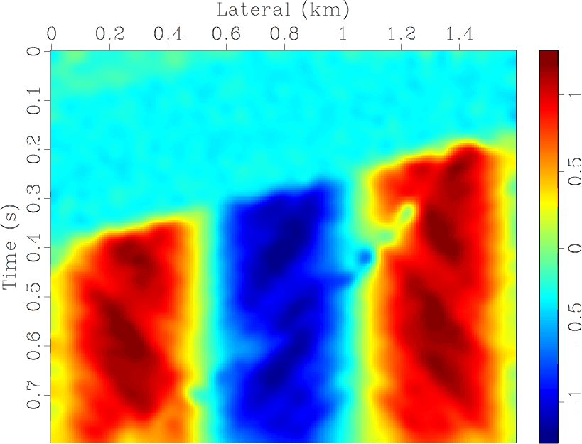
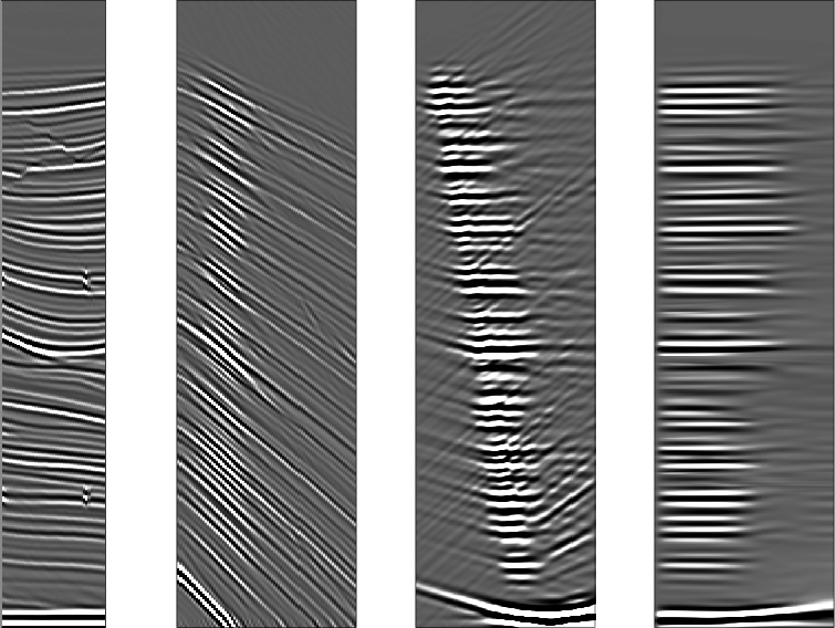
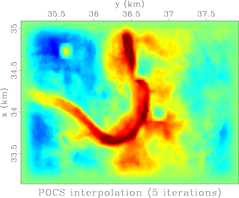
By default, sfgrey displays the first axis running vertical from top to bottom, which corresponds to transp=y yreverse=y and is a common way to display seismic data. For other kinds of data, you can modify the default behavior by setting transp=, xreverse=, and yreverse=. The following example from geo391/hw5/pocs displays a seismic horizon using transp=y yreverse=n.

For an explanation of different color schemes (specified with color= parameter), please refer to previous posts:

• Tutorial on colormaps
• Light Bartlein color palette
• Cube-helix color palette
• User-defined color palettes
• Standard color palettes

10 previous programs of the month:

• sfhistogram
• sfmf
• sfbin
• sfthreshold
• sfsigmoid
• sfmax1
• sfstolt
• sfltft
• sfeikonal
• sfhelicon