A new paper is added to the collection of reproducible documents: Multi-channel quality factor Q estimation

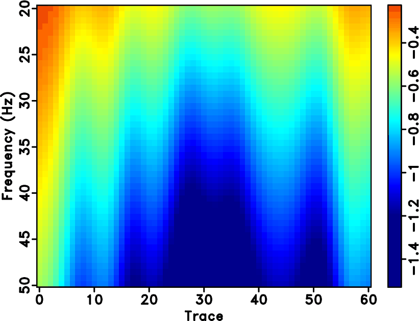
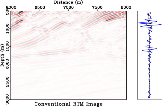
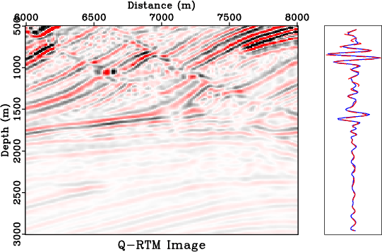
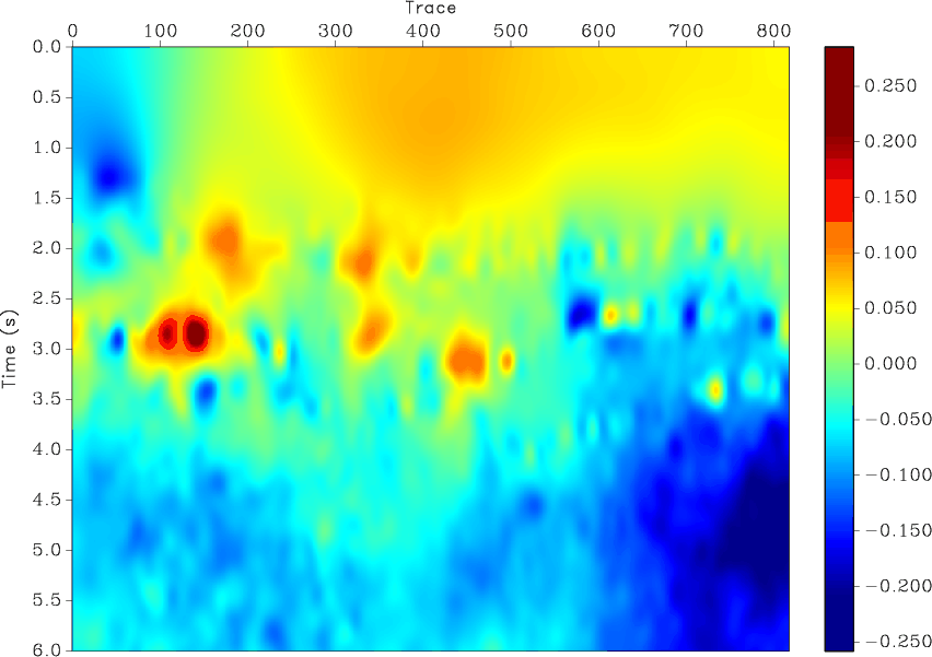
The estimation of quality factor, Q, plays an important role in many geophysical problems, including Q-compensated seismic imaging, geophysical interpretation, and fluid characterization. One of the most widely used approaches for estimating Q is the spectral ratio method (SRM). However, the spectral division in SRM may not be stable due to the spectral nulls. The shaping regularized inversion that treats the spectral division as a regularized least-squares inversion problem can help solve the spectral-nulls problem and make the spectral division stable. In the case of very noisy seismic data, the time-frequency maps can not be optimally obtained and thus the Q estimation performance will be strongly affected and unstable even with the regularized inversion method. We propose a multi-channel Q estimation approach that takes advantage of the multi-channel spatial coherence to constrain the inversion so that the estimated Q is spatially continuous. We use a set of synthetic and real data examples to demonstrate the performance of the multi-channel Q estimation method. Results show that the proposed method can obtain accurate and more importantly stable Q estimation result even in the case of strong random noise.

A new paper is added to the collection of reproducible documents: Deblending of simultaneous-source data using a structure-oriented space-varying median filter

In seismic data processing, the median filter is usually applied along the structural direction of seismic data in order to attenuate erratic or spike-like noise. The performance of a structure-oriented median filter highly depends on the accuracy of the estimated local slope from the noisy data. When local slope contains significant error, which is usually the case for noisy data, the structure-oriented median filter will still cause severe damages to useful energy. We propose a type of structure-oriented median filter that can effectively attenuate spike-like noise even when the local slope is not accurately estimated, which we call structure-oriented space-varying median filter. A structure-oriented space-varying median filter can adaptively squeeze and stretch the window length of the median filter when applied in the locally flattened dimension of an input seismic data in order to deal with the dipping events caused by inaccurate slope estimation. We show the key difference among different types of median filters in detail and demonstrate the principle of the structure-oriented space-varying median filter method. We apply the structure-oriented space-varying median filter method to remove the spike-like blending noise arising from the simultaneous source acquisition. Synthetic and real data examples show that structure-oriented space-varying median filter can significantly improve the signal preserving performance for curving events in the seismic data. The structure-oriented space-varying median filter can also be easily embedded into an iterative deblending procedure based on the shaping regularization framework and can help obtain much improved deblending performance.

A new paper is added to the collection of reproducible documents: Viscoacoustic modeling and imaging using low-rank approximation

A constant-$Q$ wave equation involving fractional Laplacians was recently introduced for viscoacoustic modeling and imaging. This fractional wave equation has a convenient mixed-domain space-wavenumber formulation, which involves the fractional-Laplacian operators with a spatially varying power. We propose to apply low-rank approximation to the mixed-domain symbol, which enables a space-variable attenuation specified by the variable fractional power of the Laplacians. Using the proposed approximation scheme, we formulate the framework of the $Q$-compensated reverse-time migration ($Q$-RTM) for attenuation compensation. Numerical examples using synthetic data demonstrate the improved accuracy of using low-rank wave extrapolation with a constant-$Q$ fractional-Laplacian wave equation for seismic modeling and migration in attenuating media. Low-rank $Q$-RTM applied to viscoacoustic data is capable of producing images comparable in quality with those produced by conventional RTM from acoustic data.