Another old paper is added to the collection of reproducible documents:
Seismic AVO analysis of methane hydrate structures

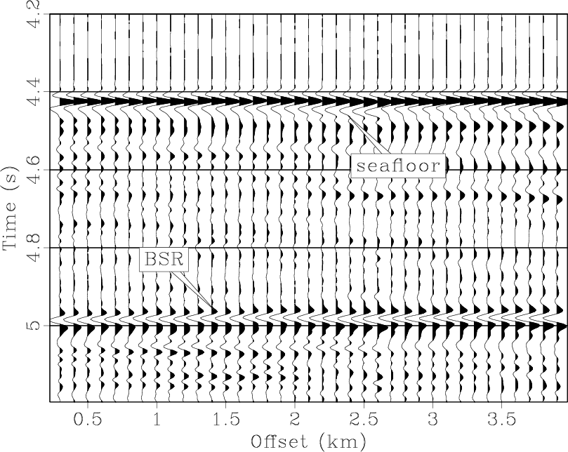
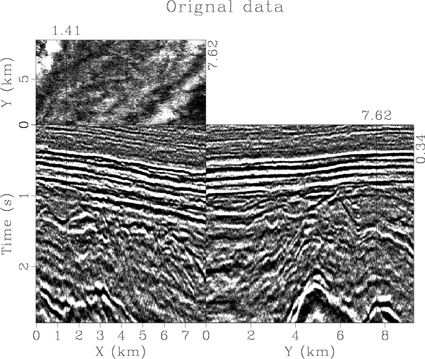
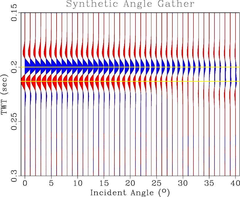
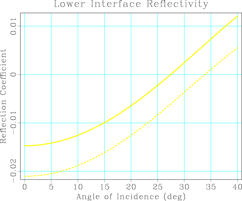
Marine seismic data from the Blake Outer Ridge offshore Florida show strong “bottom simulating reflections” (BSR) associated with methane hydrate occurence in deep marine sediments. We use a detailed amplitude versus offset (AVO) analysis of these data to explore the validity of models which might explain the origin of the bottom simulating reflector. After careful preprocessing steps, we determine a BSR model which can successfully reproduce the observed AVO responses. The P- and S-velocity behavior predicted by the forward modeling is further investigated by estimating the P- and S-impedance contrasts at all subsurface positions. Our results indicate that the Blake Outer Ridge BSR is compatible with a model of methane hydrate in sediment, overlaying a layer of free methane gas-saturated sediment. The hydrate-bearing sediments seem to be characterized by a high P-wave velocity of approximately 2.5 km/s, an anomalously low S-wave velocity of approximately 0.5 km/s, and a thickness of around 190 meters. The underlaying gas-saturated sediments have a P-wave velocity of 1.6 km/s, an S-wave velocity of 1.1 km/s, and a thickness of approximately 250 meters.

A new paper is added to the collection of reproducible documents:
Acoustic staggered grid modeling in IWAVE

IWAVE is a framework for time-domain regular grid finite difference and finite element methods. The IWAVE package includes source code for infrastructure component, and implementations of several wave physics modeling categories. This paper presents two sets of examples using IWAVE acoustic staggered grid modeling. The first set illustrates the effectiveness of a simple version of Perfectly Matched Layer absorbing boundary conditions. The second set reproduce illustrations from a recent paper on error propagation for heterogeneous medium simulation using finite differences, and demostrate the interface error effect which renders all FD methods effectively first-order accurate. The source code for these examples is packaged with the paper source, and supports the user in duplicating the results presented here and using IWAVE in other settings.

Another old paper is added to the collection of reproducible documents:
A prospect for super resolution

Wouldn’t it be great if I could take signals of 10-30 Hz bandwidth from 100 different offsets and construct a zero-offset trace with 5-100 Hz bandwidth? This would not violate Shannon’s sampling theorem which theoretically allows us to have a transform from 100 signals of 20 Hz bandwidth to one signal at 2000 Hz bandwidth. The trouble is that simple NMO is not such a transformation. Never-the-less, if the different offsets really did give us any extra information, we should be able to put the information into extra bandwidth. Let us consider noise free synthetic data and see if we can come up with a model where this could happen.

Another old paper is added to the collection of reproducible documents:
Earthquake stacks at constant offset

I show Shearer’s earthquake stacks over all source-receiver locations at constant offset and compare them to exploration seismic data. This electronic document simply reads the stacks and plots them.

A new paper is added to the collection of reproducible documents:
Adaptive prediction filtering in t-x-y domain for random noise attenuation using regularized nonstationary autoregression

Many natural phenomena, including geologic events and geophysical data, are fundamentally nonstationary. They may exhibit stationarity on a short timescale but eventually alter their behavior in time and space. We propose a 2D t-x adaptive prediction filter (APF) and further extend this to a 3D t-x-y version for random noise attenuation based on regularized nonstationary autoregression (RNA). Instead of using patching, a popular method for handling nonstationarity, we obtain smoothly nonstationary APF coefficients by solving a global regularized least-squares problem. We use shaping regularization to control the smoothness of the coefficients of APF. 3D space-noncausal t-x-y APF uses neighboring traces around the target traces in the 3D seismic cube to predict noise-free signal, so it provides more accurate prediction results than the 2D version. In comparison with other denoising methods, such as frequency-space deconvolution, time-space prediction filter, and frequency-space RNA, we test the feasibility of our method in reducing seismic random noise on three synthetic datasets. Results of applying the proposed method to seismic field data demonstrate that nonstationary t-x-y APF is effective in practice.

This reproducible paper is the first direct contribution from Jilin University, China.