sfkirmigsr implements 2-D Kirchoff prestack depth migration (PSDM).

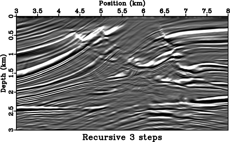
The following example from tccs/eikods/marm shows an application of sfkirmigsr to imaging synthetic Marmousi data.

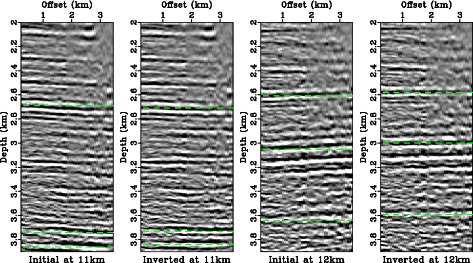
With cig= flag, the program can output common-image gathers, as in the followung example from tccs/time2depth2/beinew:

The traveltimes needed for Kirchhoff migration are computed externally and supplied in the form of traveltime tables stable= and rtable=. To increase accuracy, additional information can be provided by traveltime derivatives sderive= and rderiv=, as explained in the paper
Kirchhoff migration using eikonal-based computation of traveltime source-derivatives.

Other useful parameters are antialias= (for controling antialiasing) and aperture= (for controling migration aperture).

The program also has the adjoint flag adj=, which makes it suitable for least-squares inversion.

10 previous programs of the month:

• sfsnr2
• sflpf
• sfslice
• sfzomig3
• sfseislet
• sfmig2
• sfsort
• sfdivn
• sfpldb and sfplas
• sfisolr2

Matplotlib is a popular Python library for 2D plotting, which emulates (and exceeds) the plotting functionality of MATLAB.

At the Madagascar Working Workshop in 2018, a couple of new scripts were added to simplify plotting with Matplotlib in Madagascar.

• sfmatplotlib can be used to plot RSF files.You can use it as follows:
  sfmatplotlib <matplotlib function> <plot options> [format=eps] < inp.rsf [ > out.eps] 
  

  Without the standard output, the figure is displayed on the screen.

  

  The figure above was generated with

  sfspike n1=1000 k1=300 | sfbandpass fhi=2 phase=y| sfmatplotlib plot title="Welcome to Maagascar" grid=y linewidth=3 format=png > figure.png
  

  Futher enhancements are possible.

• sfpgreywfl is a script contributed by Carlos da Costa that uses matplotlib for plotting a seismic wavefiels overlaid on the velocity model.
  

  The figure above was generated with

  sfpgreywfl < wavefield.rsf bg=velocity.rsf wflcmap=seismic title="Wavefield" barlabel="Velocity (m/s)" tmin=0.08 savefile=figure.gif
  

scons2jupyter is a simple script that converts a Madagascar-style SConstruct file to a Jupyter notebook with a Python interface.

You can use it by simply running

scons2jupyter < SConstruct > mynotebook.ipynb

An example notebook is the result of running scons2jupyter in bei/vela/vscan.

A newly created notebook can be populated with Markdown text and explanations to implement the discipline of literate programmins.

sfsnr2 computes the signal-to-noise (SNR) ratio in decibells.

The following example from tccs/intshape/fsyn uses the SNR computation to compare the convergence of two different methods.

SNR is computed according to the equation

$SNR=\displaystyle 10\log_{10}\left(\frac{\Arrowvert \mathbf{s} \Arrowvert_2^2}{\Arrowvert\mathbf{n}\Arrowvert_2^2}\right)$

The signal vector $\mathbf{s}$ is in the standard input, the noise vector $\mathbf{n}$ is in the file specified by noise= parameter.

10 previous programs of the month:

• sflpf
• sfslice
• sfzomig3
• sfseislet
• sfmig2
• sfsort
• sfdivn
• sfpldb and sfplas
• sfisolr2
• sfsimilarity

sfslpf estimates a non-stationary filter using shaping regularization.

The method is described in the reproducible paper Adaptive multiple subtraction using regularized nonstationary regressio

The following example from tccs/lpf/plut shows a common-offset section from the Pluto synthetic dataset before and after adaptive multiple subtraction with the help of sflpf.

Given target data $m(\mathbf{x})$ (specified with match= parameter) and a collection of fitting functions $s_k(\mathbf{x})$ (specified in the standard input), sflpf finds the fitting coefficients $b_k(\mathbf{x})$ by minimizing the error

$m(\mathbf{x}) – \displaystyle \sum_{k=1}^{N} b_k(\mathbf{x})\,s_k(\mathbf{x})$

while constraining the coefficients to be smooth. The smoothness is controlled by rect#= parameters, as in sfsmooth.

Shaping regularization is carried out iteratively, niter= controls the number of iterations.

The mean coefficient from the example above is shown in the figure below.

Optionally, a prediction-error filter can be applied to whiten the residual. The filter is specified with the help of pef= and lag= parameters, with a multidimensional helical filter specified as in sfhelicon.

The complex version of the same program is sfclpf.

10 previous programs of the month:

• sfslice
• sfzomig3
• sfseislet
• sfmig2
• sfsort
• sfdivn
• sfpldb and sfplas
• sfisolr2
• sfsimilarity
• sfmutter

sfslice extracts a slice from the data given by a curve (in 2-D) or a surface (in 3-D).

The right plot in the following example from gee/prc/bob shows the semblance extracted using sfslice from the semblance scan along the trajectory picked with sfpick.

sfslice does not have parameters other than pick=, which points to the file with the surface for extraction.

It performs a simple linear interpolation to extract the values.

10 previous programs of the month:

• sfzomig3
• sfseislet
• sfmig2
• sfsort
• sfdivn
• sfpldb and sfplas
• sfisolr2
• sfsimilarity
• sfmutter
• sfintbin

sfbargraph is a new plotting program for displaying data as bars.

The bottom plot in the figure below shows a simple example from rsf/rsf/sfnoise.

The unique parameters of sfbargraph include width= for controling the relative width of the bars and stack= to control if the bars from multiple input traces should be stacked on top of one another.

The other parameters are shared with other plotting programs.

sfzomig3 performs 3-D zero-offset modeling or migration using one-way wave extrapolation and the exploding reflector concept.

The following example from rsf/su/rsflab10 shows the result of migrating the benchmark Viking Graben dataset.

The algorithm used by sfzomig3 is known as extended split-step or phase-shift plus interpolation (PSPI). It works in the frequency domain and mixed space-wavenumber domain.

• Gazdag, J., and Sguazzero, P., 1984, Migration of seismic data by phase shift plus interpolation: Geophysics, 49, 124-131.
• Kessinger, W., 1992, Extended split-step Fourier migration: 62nd Ann.
  Internat. Mtg., Soc. Expl. Geophys., Expanded Abstracts, 917-920.

Depending on inv= flag, sfzomig3 performs modeling or migration (if mode=m) or datuming (upward or downward) wavefield continuation (if mode=d). The default is migration (mode=m inv=n).

The algorithm efficiency depends on the number of reference velocities, which corresponds to the number of spatial Fourier transforms. By default, the algorithm is trying to estimate this number automatically at each depth step. The maximum number can be set by nrmax=.

The pmx=, pmy=, and tmx=, tmy= parameters control padding and tapering in space, needed to avoid boundary reflections and Fourier wrap-around artifacts.

10 previous programs of the month:

• sfseislet
• sfmig2
• sfsort
• sfdivn
• sfpldb and sfplas
• sfisolr2
• sfsimilarity
• sfmutter
• sfintbin
• sfbox

sfseislet implements the 2-D seislet transform.

The seislet transform theory is descibed in the paper Seislet transform and seislet frame.

The following example from fpwd/teapot shows a 3-D seismic image before and after a seislet transform in the inline direction.

To perform the forward seislet transform, run sfseislet with the flag adj=y. To run the inverse transform, use adj=n. In a confusing choice of parameter names, inv= does not control the direction of the transform but the type of the weighting function used. Another control is provided by unit=.

A required auxiliary input is the dip field specified by dip=. If the dip was estimated using plane-wave destruction (sfdip), the order= parameter should be the same.

Different types of the seislet transform (specified by type=) correspond to different types of the corresponding digital wavelet transform. The choices are haar, linear, and biorthogonal.

10 previous programs of the month:

• sfmig2
• sfsort
• sfdivn
• sfpldb and sfplas
• sfisolr2
• sfsimilarity
• sfmutter
• sfintbin
• sfbox
• sfslant

sflinear performs 1-D linear interpolation of irregularly spaced data.

The following example from rsf/su/rsflab4 shows a linearly interpolated velocity profile:

The input to sflinear contains coordinate-value pairs arranged so that the second dimension of the data is n2=2. The output contains regularly sampled values on the specified grid.

If the input coordinates are not in order and need sorting, use sort=y.

The output grid can be specified either by supplying it in a pattern file pattern= or by specifying the usual parameters n1=, o1=, d1=.

If the number of iterations specified by niter= is greater than zero, sflinear switches from simple linear interpolation to iterative interpolation by shaping regularization, which can produce a smooth output. The additional parameters to control this process are nw= (size of the local Lagrange interpolation filter for forward interpolation) and rect= (smoothing radius for shaping).

10 previous programs of the month:

• sfmig2
• sfsort
• sfdivn
• sfpldb and sfplas
• sfisolr2
• sfsimilarity
• sfmutter
• sfintbin
• sfbox
• sfslant