The example in rsf/tutorials/well-tie reproduces the tutorial from Evan Bianco on well-tie calculus. The tutorial was published in the June 2014 issue of The Leading Edge.


Madagascar users are encouraged to try improving the results.
Tutorial on well-tie calculus
June 26, 2015 Examples No comments
Similarity-weighted semblance
June 25, 2015 Documentation No comments
A new paper is added to the collection of reproducible documents:
Velocity analysis using similarity-weighted semblance

Weighted semblance can be used for improving the performance of the traditional semblance for specific datasets. We propose a novel approach for prestack velocity analysis using weighted semblance. The novelty comes from a different weighting criteria in which the local similarity between each trace and a reference trace is used. On one hand, low similarity corresponds to a noise point or a point indicating incorrect moveout, which should be given a small weight. On the other hand, high similarity corresponds to a point indicating correct moveout, which should be given a high weight. The proposed approach can also be effectively used for analyzing AVO anomalies with increased resolution compared with AB semblance. Both synthetic and field CMP gathers demonstrate higher resolution using the proposed approach. Applications of the proposed method on a prestack dataset further confirms that the stacked data using the similarity-weighted semblance can obtain better energy-focused events, which indicates a more precise velocity picking.
Test case for PEF estimation
June 24, 2015 Documentation No comments
Another old paper is added to the collection of reproducible documents:
Test case for PEF estimation with sparse data II
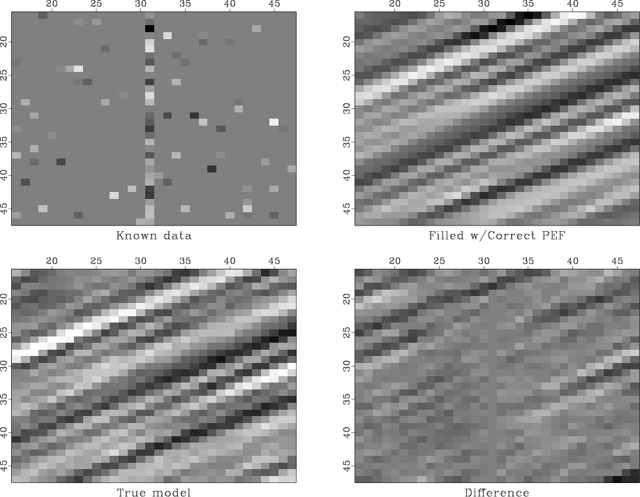
The two-stage missing data interpolation approach of Claerbout (1998) (henceforth, the GEE approach) has been applied with great success (Fomel et al., 1997; Clapp et al., 1998; Crawley, 2000) in the past. The main strength of the approach lies in the ability of the prediction error filter (PEF) to find multiple, hidden correlation in the known data, and then, via regularization, to impose the same correlation (covariance) onto the unknown model. Unfortunately, the GEE approach may break down in the face of very sparsely-distributed data, as the number of valid regression equations in the PEF estimation step may drop to zero. In this case, the most common approach is to simply retreat to regularizing with an isotropic differential filter (e.g., Laplacian), which leads to a minimum-energy solution and implicitly assumes an isotropic model covariance.
A pressing goal of many SEP researchers is to find a way of estimating a PEF from sparse data. Although new ideas are certainly required to solve this interesting problem, Claerbout (2000) proposes that a standard, simple test case first be constructed, and suggests using a known model with vanishing Gaussian curvature. In this paper, we present the following, simpler test case, which we feel makes for a better first step.
- Model: Deconvolve a 2-D field of random numbers with a simple dip filter, leading to a “plane-wave” model.
- Filter: The ideal interpolation filter is simply the dip filter used to create the model.
- Data: Subsample the known model randomly and so sparsely as to make conventional PEF estimation impossible.
We use the aforementioned dip filter to regularize a least squares estimation of the missing model points and show that this filter is ideal, in the sense that the model residual is relatively small. Interestingly, we found that the characteristics of the true model and interpolation result depended strongly on the accuracy (dip spectrum localization) of the dip filter. We chose the 8-point truncated sinc filter presented by Fomel (2000). We discuss briefly the motivation for this choice.
Reproducible research and PDF files
June 21, 2015 Systems No comments
Claerbout’s principle of reproducible research, as formulated by Buckheit and Donoho (1995), states:
An article about computational science in a scientific publication is not the scholarship itself, it is merely advertising of the scholarship. The actual scholarship is the complete software development environment and the complete set of instructions which generated the figures.
The geophysics class in the SEGTeX package features a new option: reproduce, which attaches SConstruct files or other appropriate code (Matlab scripts, Python scripts, etc.) directly to the PDF file of the paper, with a button under every reproducible figure for opening the corresponding script. Unfortunately, not every PDF viewer supports this kind of links. The screenshot below shows evince viewer on Linux, where clicking the button opens the file with gedit editor. 
Double-elliptic approximation in TI media
June 16, 2015 Documentation No comments
Another old paper is added to the collection of reproducible documents:
The double-elliptic approximation in the group and phase domains
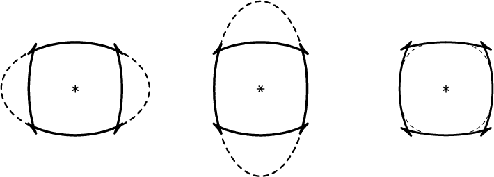
Elliptical anisotropy has found wide use as a simple approximation to transverse isotropy because of a unique symmetry property (an elliptical dispersion relation corresponds to an elliptical impulse response) and a simple relationship to standard geophysical techniques (hyperbolic moveout corresponds to elliptical wavefronts; NMO measures horizontal velocity, and time-to-depth conversion depends on vertical velocity). However, elliptical anisotropy is only useful as an approximation in certain restricted cases, such as when the underlying true anisotropy does not depart too far from ellipticity or the observed angular aperture is small. This limitation is fundamental, because there are only two parameters needed to define an ellipse: the horizontal and vertical velocities. (Sometimes the orientation of the principle axes is also included as a free parameter, but usually not.)
In a previous SEP report Muir (1990) showed how to extend the standard elliptical approximation to a so-called double-elliptic form. (The relation between the elastic constants of a TI medium and the coefficients of the corresponding double-elliptic approximation is developed in a companion paper, (Muir, 1991).) The aim of this new approximation is to preserve the useful properties of elliptical anisotropy while doubling the number of free parameters, thus allowing a much wider range of transversely isotropic media to be adequately fit. At first glance this goal seems unattainable: elliptical anisotropy is the most complex form of anisotropy possible with a simple analytical form in both the dispersion relation and impulse response domains. Muir’s approximation is useful because it nearly satisfies both incompatible goals at once: it has a simple relationship to NMO and true vertical and horizontal velocity, and to a good approximation it has the same simple analytical form in both domains of interest.
The purpose of this short note is to test by example how well the double-elliptic approximation comes to meeting these goals:
- Simple relationships to NMO and true velocities on principle axes.
- Simple analytical form for both the dispersion relation and impulse response.
- Approximates general transversely isotropic media well.
The results indicate that the method should work well in practice.
Program of the month: sfintbin
June 10, 2015 Celebration No comments
sfintbin uses trace headers to arrange input traces in a 3-D cube.
The input to this program typically comes from reading a SEGY file with sfsegyread.
The following example from tccs/phase/boon3 shows a typical output:

sfintbin takes as an input a 2-D trace file and its corresponding trace header file (specified by head=). The header file is assumed to contain integer values. The output 3-D cube is generated according to trace header keys, which can be specified by name (xk=, yk=) or by number (xkey=, ykey=). In the example above, the parameters are xk=cdp and yk=fldr. If you are unsure which keys to use, try sfheaderattr. The range of values can be controlled with xmin=, xmax=, ymin=, ymax=.
sfintbin performs a very simple operation: it goes through the input file and assigns traces to the output according to their header keys. If there are several traces with the same x and y keys, the last one survives. If there are bins in the output with no input, they are filled with zeros. You can output the mask of empty traces using mask=. You can output the mapping of traces using map=. The latter is particularly useful for the inverse operation (mapping from 3-D back to 2-D), which can be performed with inv=y.
For an absent trace header key, which corresponds to a trace number in a gather, you can set xkey= to a negative number. For this to work, the input needs to be sorted in the corresponding gathers, which can be accomplished with sfheadersort.
To produce a 4-D output (for example, a set of gathers in 3-D), try sfintbin3.
10 previous programs of the month:
Literate programming with IPython notebooks
June 2, 2015 Systems No comments
 Literate programming is a concept promoted by Donald Knuth, the famous computer scientist (and the author of the Art of Computer Programming.) According to this concept, computer programs should be written in a combination of the programming language (the usual source code) and the natural language, which explains the logic of the program.
When it comes to scientific programming, using comments for natural-language explanations is not always convenient. Moreover, it is limited, because such explanations may require figures, equations, and other common elements of scientific texts. IPython/Jupyter notebooks provide a convenient tool for combining different text elements with code. See the notebook at https://github.com/sfomel/ipython/blob/master/LiterateProgramming.ipynb for an example on how to implement literate programming using an IPython notebook with reproducible SConstruct data-analysis workflows in Madagascar.
Related posts:
* Madagascar in the cloud
* Reproducible research and IPython notebooks