sfkirmod is a program for modeling seismic reflection data using the Kirchhoff method. According to this method, the reflection response is computed by integrating over the reflector surface. For a theoretical derivation, see, for example,

Haddon, R. A. W., and P. W. Buchen, 1981, Use of Kirchhoff’s formula for body wave calculations in the earth: Geophys. J. Roy. Astr. Soc., 67, 587-598.

At the moment, sfkirmod can handle only asymptotic Green’s functions, analytically computed in three kinds of velocity models:

1. Constant velocity
2. Constant gradient of velocity
3. Constant gradient of velocity squared

The type is specified with type= parameter, and the velocity model is specified with vel=, refx=, refz=, gradx=, and gradz=.

The following example from rsf/scons/rsf shows shot gathers modeled by sfkirmod in a medium with horizontal reflectors and a constant vertical gradient of velocity

It is also possible to model a converted (PS or SP) wave by supplying vel2=, gradx2=, and gradz2= to specify the converted velocity. The standard input file for sfkirmod contains the shape of one or more reflectors. Several other input files can be optionally provided: dip= specifies the slope of the reflector(s), refl= specifies normal-incidence reflectivity (AVA intercept), rgrad= specifies AVA gradient.

The sampling of the time axis in the output is controlled by nt=, t0=, and dt= parameters. A Ricker wavelet is used with the peak frequency specified by freq=. Factors such as the geometrical spreading and the obliquity factor are taken into account. The geometrical spreading correction is different for 2-D (cylindrical waves) or 2.5-D (spherical waves). The default behavior is 2.5_D. To switch to 2-D, use twod=y. By default, sfkirmod outputs shot gathers.

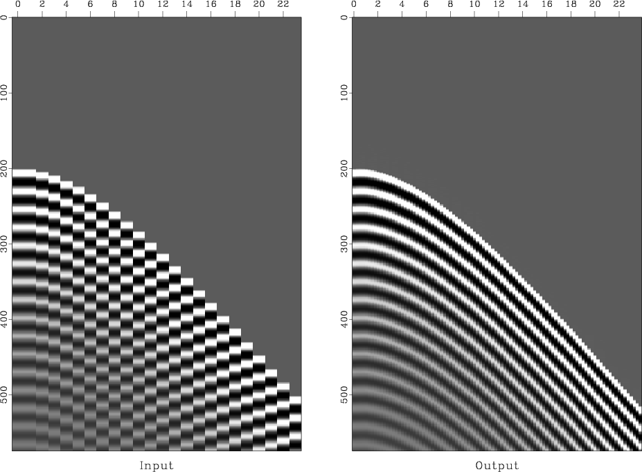
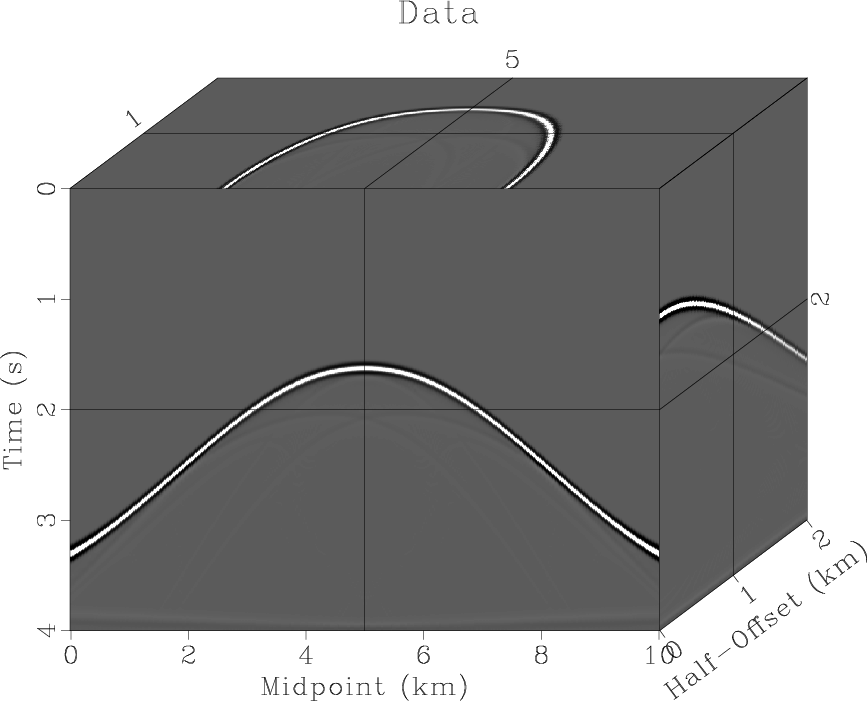
It is also possible to compute CMP gathers directly by using cmp=y. The following example from jsg/crs/dome2 shows CMP gathers computed over a hyperbolic-shape reflector.

Since Kirchhoff modeling is fundamentally a linear operation, it is easy to run sfkirmod in a data-parallel fashion, for example by using pscons with split=[1,n1] and reduce=’add’.

The 3-D version of sfkirmod is sfkirmod3.

10 previous programs of the month

• sfiwarp
• sfpick
• sffft3
• sfdip
• sfderiv
• sfgrey3
• sfspectra
• sfnoise
• sfgraph
• sfclip

sfiwarp performs mapping between different coordinates.

If you have sampled functions $f(x)$ and $y(x)$, sfiwarp with inv=y (the default) finds sampled $f(y)$. If inv=n, sfiwarp takes $f(y)$ and $y(x)$ and finds $f(x)$. In both cases, the sampled $y(x)$ function is supplied in a file specified by warp= parameter. The following example from milano/taupvel/cmp shows a seismic taup-p gather flattening by predictive painting and time warping.

Coordinate mapping is a fundamental data-transformation operation, which finds many applications. The term warping comes from medical imaging. See, for example,

• Wolberg, G., 1990, Digital image warping: IEEE Computer Society Press.
• W. Burnett and S. Fomel, 2009, Moveout analysis by time-warping: 79th Annual International Meeting, SEG, 3710-3714.

The algorithm used in sfiwarp is B-spline interpolation and inverse spline interpolation. If forward warping (inv=n) is $\mathbf{f}_x = \mathbf{B}\,\mathbf{f}_y$, then the inverse transformation (inv=y) is given by the regularized least-squares inverse
$$\mathbf{f}_y = \left(\mathbf{B}^T\,\mathbf{B} + \epsilon^2\,\mathbf{D}\right)^{-1}\,\mathbf{B}^T\,\mathbf{f}_x\;,$$ where $\mathbf{D}$ is the derivative operator. The $\epsilon$ parameter is supplied by eps=. The sampling in $y$ is supplied by n1=, d1=, o1= parameters.

For 2-D and 3-D versions, try sfiwarp2 and sfiwarp3.

10 previous programs of the month

• sfpick
• sffft3
• sfdip
• sfderiv
• sfgrey3
• sfspectra
• sfnoise
• sfgraph
• sfclip
• sfagc

sfpick performs automatic picking from semblance-like panels.

The underlying algorithm is described in Appendix B of the paper Velocity analysis using AB semblance and is inspired by the method of virtual endoscopy in medical imaging. The following example from tccs/avo/avo shows an automatic pick through AB semblance.

If smooth=n, the program picks an optimal path through the panel but does not try to smooth it. If smooth=y (the default), the picked path is additionally smoothed using shaping regularization. The smoothing radius across different dimensions is controled by rect1=, rect2=, etc. parameters. The number of shaping iterations is specified by niter=. The following example from sep/vc2/beivc shows two different picks for two different values of the rect1= parameter

The vel0= refers to the value the pick initially takes at the surface (the origin). This value is not necessarily preserved, because it can get modified by smoothing. In the following example from tccs/timelapse/timelapse, vel0=1.

The an= parameter controls the anisotropy between the two axes of the semblance panel. Varying this parameter, you can achieve picks that are more rigid or more flexible. The gate= parameter controls how far (in velocity samples) the pick can swing between two neighboring time samples. Changing its value also affects the flexibility of the picked trend.

For picking from 3-D (rather than 2-D) panels, try sfpick3.

10 previous programs of the month

• sffft3
• sfdip
• sfderiv
• sfgrey3
• sfspectra
• sfnoise
• sfgraph
• sfclip
• sfagc
• sfenvelope

sffft3 implements a complex-to-complex Fast Fourier Transform (FFT) along an arbitrary axis.

The FFT library that Madagascar uses by default is KISS FFT, created by Mark Borgerding. KISS stands for Keep it simple, Stupid! KISS FFT may not be as fast as FFTW but it is lightweight and easy to include in the distribution.

The axis= parameter specifies the data axis for performing the transform. The following example from bei/ft1/plane4 (Jon Claerbout’s Basic Earth Imaging) shows different forms of the Fourier transform applied to a 2-D dataset.

The algorithm in KISS FFT uses a mixed-radix algorithm, which is most efficient when the input size is $N=2^k\,3^l\,5^m$. By default, the input data is padded to the next optimal size, additionally multiplied by 2. To disable this behavior, use opt=n pad=1.

By default, sffft3 applies no scaling in the forward transform and $1/N$ scaling in the inverse transform. To apply a symmetric $1/\sqrt{N}$ scaling in both cases, use sym=y.

For a real-to-complex FFT along the first axis, use sffft1.

For a real-to-real Cosine Fourier Transform, use sfcosft.

To apply FFT as a linear operator, try sffft wrapper script.

10 previous programs of the month:

• sfdip
• sfderiv
• sfgrey3
• sfspectra
• sfnoise
• sfgraph
• sfclip
• sfagc
• sfenvelope
• sfcontour

sfdip estimates a local slope (dip) using the plane-wave destruction algorithm.

The dip is measured in time samples. If $\alpha$ is the dip angle, then the output of sfdip corresponds to the dimensionless quantity $p=\tan{\alpha}$.

The following example from jsg/flat/flat shows an input synthetic dataset and an estimated dip field

When applied to 3-D data, sfdip outputs a 4-D file with n4=2 and two dips (inline and crossline). To compute only the inline dip, use n4=0. To compute only the crossline dip, use n4=1. The following example from sep/plane/qint shows an input synthetic 3-D dataset and the two dip components calculated from it.

The algorithm consists of a number of non-linear Gauss-Newton iterations (specified by niter=) with a number of linear CG-shaping iterations (specified by liter=) inside each non-linear cycle. The convergence depends on the initial dip values, which can be specified either as constants (p0= and q0=) or as auxiliary input files (idip= and xdip=). If it is necessary to constrain the range of dip values, it can be controlled by specifying minimum or maximum parameters (pmin=, pmax= and qmin=, qmax=). The smoothness of the dip is assured by shaping regularization and controled by the smoothing radii rect1=, rect2=, rect3=.

With default parameters, the dip estimate is accurate only up to 45 degrees. To estimate steeper (aliased) dips, increase the order= parameter. The order of the filter corresponds to the maximum dip. Alternatively, one can use the technique of filter stretching (interlacing), explained by Claerbout; the stretching parameters are nj1= and nj2=. The following examples from sep/pwd/alias show aliased data interpolation using (a) order=12 (b) order=3 nj1=4.

For a faster version, with only one non-linear iteration but with fewer options, try sffdip. To estimate two interfering dips, try sftwodip2. To estimate a number of constant dips, try sfdips.

10 previous programs of the month

• sfderiv
• sfgrey3
• sfspectra
• sfnoise
• sfgraph
• sfclip
• sfagc
• sfenvelope
• sfcontour
• sfsmooth

sfderiv applies the first derivative filter.

The algorithm implemented in this program is described in the paper

Pei, S.-C., and P.-H. Wang, 2001, Closed-form design of maximally flat FIR Hilbert transformers, differentiators, and fractional delayers by power series expansion: IEEE Trans. on Circuits and Systems, v. 48, No. 4, 389-398.

It is based on the Taylor expansion of the inverse sine function
$$\arcsin{x} = \displaystyle \sum_{n=0}^{\infty} \frac{(2n)!}{4^n\,(n!)^2\,(2n+1)}\,x^{2n+1}$$
which turns into an expansion of the ideal derivative filter into a chain of digital filters. The order= parameter controls the order of the expansion and the accuracy-efficiency trade-off. The following example from rsf/rsf/sfderiv shows the frequency responses and the impulse responses for differentiators of different orders

An alternative is sfigrad, which implements a simple first-order derivative. igrad is more efficient and adequate when computing derivatives of smooth functions.

Previous programs of the month

• sfgrey3
• sfspectra
• sfnoise
• sfgraph
• sfclip
• sfagc
• sfenvelope
• sfcontour
• sfsmooth

sfgrey3 generates “cube” plots from 3-D data. A cube plot displays sections from a 3-D cube as faces of the cube.

Some of the options specific to this kind of display are:

• flat= The flat parameter tells sfgrey3 whether to display the cube as a flat image or in a 3-D projection. The default is flat=y. The following example from bei/fld/cube displays the same input data with both options:

• frame1=, frame2=, frame3= The frame parameters select the slices from the cube to be displayed in the plot. The default is to take the first slice from the vertical and the out-of-plane axis (frame1=0 frame3=0) and the last slice from the horizontal axis (frame2=n2-1). In the following example from geo384w/hw3/gulf, the data size is n1=1000 n2=250 n3=48 and the frame parameters are frame1=500 frame2=160 frame3=10:

• point1=, point2= The point1= and point2= parameters control the aspect ratio of the cube by specifying the ratio (from 0 and 1) that the front face of the cube takes from the plot in the vertical and the horizontal dimension, respectively. The default is point1=0.5 point2=0.5. The following example from sep/plane/qint has point1=0.85 point2=0.74:

• movie= The movie parameter allows the user to create a movie looping over slices in a cube instead of a static picture. The value of the parameter (from 1 to 3) indicates the axis for looping or 0 (the default) for no movie. The frame increment in the movie is controled by dframe=. The following example from cwp/geo2009TTIModeSeparation/tti3 uses movie=1 to loop over the vertical axis:

To generate a movie out of 4-D data, you can use sfgrey4. Here is an example:

Previous programs of the month:

• sfspectra
• sfnoise
• sfgraph
• sfclip
• sfagc
• sfenvelope
• sfcontour
• sfsmooth

sfspectra computes spectrum, the absolute value of the 1-D Fourier transform along the fast axis.

The following example from rsf/su/rsfkasper shows a seismic shot gather before and after high-pass filtering and the corresponding spectra computed with sfspectra.

sfspectra has only one option: all=. If all=n (the default behavior), the spectrum is computed separately for each trace. If all=y, the output is the spectrum averaged across all traces.

For a two-dimensional version, try sfspectra2. The following figures from jsg/seislet/lena show the infamous Lena image and the “seismic Lena” (after Chris Liner and David Monk)

and the corresponding 2-D spectra computed with sfspectra2

Previous programs of the month

• sfnoise
• sfgraph
• sfclip
• sfagc
• sfenvelope
• sfcontour
• sfsmooth

tkvpconvert provides a Tkinter GUI (graphical user interface) for vpconvert. It is a silly exercise, which simply demonstrates an ability to generate specialized GUIs for Madagascar scripts and programs.

sfsmooth, one of the most useful Madagascar programs, implements smoothing by triangle filtering.

The idea of triangle filtering is explained in Jon Claerbout’s books Processing versus Inversion and Image Estimation by Example. You can find the explanation in the chapter Smoothing with box and triangle. The triangle filter of radius is a correlation of two box filters. In the Z-transform notation,
$$T_k(Z) = B_k(1/Z)\,B_k(Z)$$
where
$$B_k(Z) = \displaystyle \frac{1}{k}\,\left(1+Z+Z^2+\cdots+Z^k\right) = \frac{1}{k}\,\frac{1-Z^{k+1}}{1-Z}$$
and $k$ is the smoothing radius. Triangle filtering is a very efficient operation, because it requires only $N$ multiplications for the input of size $N$.

Triangle filtering serves as a good approximation to more expensive Gaussian filtering. Repeated triangle filtering rapidly approaches Gaussian filtering (a consequence of the central limit theorem). The following example from jsg/shape/smoo demonstrates how repeated application of triangle smoothing turns a triangle filter into a Gaussian filter

The following example from gee/ajt/triangle demonstrated how sfsmooth handles boundary conditions: the energy is reflected from the side in order to preserve the zero-frequency (DC) component of the input signal. Repeated smoothing or smoothing with a very large radius turns every signal into a constant.

In multiple dimensions, triangle smoothing is applied sequentially in different directions, possible with different radii (controlled by rect#= ) parameter. The following example from gee/ajt/mound shows shapes created by 2-D triangle smoothing after one pass and two passes (repeat=2).

Triangle smoothing is theoretically a self-adjoint operator. Numerically, the adjoint and forward operators are different. The action is controlled by the adj= parameter.

For smoothing with a box instead of a triangle, use sfboxsmooth.

For a different approach to smoothing, try sfgaussmooth, which implements smoothing by recursive Gaussian filtering.

Previous programs of the month

• sfnoise
• sfgraph
• sfclip
• sfagc
• sfenvelope
• sfcontour