Month: July 2019

Low-rank viscoacoustic wave extrapolation

July 18, 2019 Documentation No comments

A new paper is added to the collection of reproducible documents: Viscoacoustic modeling and imaging using low-rank approximation

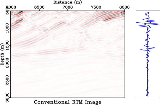
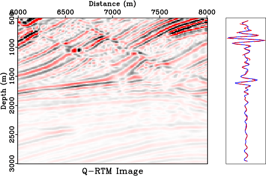
A constant-$Q$ wave equation involving fractional Laplacians was recently introduced for viscoacoustic modeling and imaging. This fractional wave equation has a convenient mixed-domain space-wavenumber formulation, which involves the fractional-Laplacian operators with a spatially varying power. We propose to apply low-rank approximation to the mixed-domain symbol, which enables a space-variable attenuation specified by the variable fractional power of the Laplacians. Using the proposed approximation scheme, we formulate the framework of the $Q$-compensated reverse-time migration ($Q$-RTM) for attenuation compensation. Numerical examples using synthetic data demonstrate the improved accuracy of using low-rank wave extrapolation with a constant-$Q$ fractional-Laplacian wave equation for seismic modeling and migration in attenuating media. Low-rank $Q$-RTM applied to viscoacoustic data is capable of producing images comparable in quality with those produced by conventional RTM from acoustic data.

Program of the month: sflpf

July 9, 2019 Programs No comments

sfslpf estimates a non-stationary filter using shaping regularization.

The method is described in the reproducible paper Adaptive multiple subtraction using regularized nonstationary regressio

The following example from tccs/lpf/plut shows a common-offset section from the Pluto synthetic dataset before and after adaptive multiple subtraction with the help of sflpf.

Given target data $m(\mathbf{x})$ (specified with match= parameter) and a collection of fitting functions $s_k(\mathbf{x})$ (specified in the standard input), sflpf finds the fitting coefficients $b_k(\mathbf{x})$ by minimizing the error

$m(\mathbf{x}) – \displaystyle \sum_{k=1}^{N} b_k(\mathbf{x})\,s_k(\mathbf{x})$

while constraining the coefficients to be smooth. The smoothness is controlled by rect#= parameters, as in sfsmooth.

Shaping regularization is carried out iteratively, niter= controls the number of iterations.

The mean coefficient from the example above is shown in the figure below.

Optionally, a prediction-error filter can be applied to whiten the residual. The filter is specified with the help of pef= and lag= parameters, with a multidimensional helical filter specified as in sfhelicon.

The complex version of the same program is sfclpf.

10 previous programs of the month: