Opinion poll

September 26, 2012 Links No comments

A post-meeting survey after the 2012 Madagascar School in Austin showed an overwhelmingly positive response. 100% of those who responded to the survey said that they would attend events like that in the future (one person said “Sure. If it takes part in my home country.“, another one added “I think is the best open source project out there. I think that is not because of the programs (which are very good) themselves but because of the community and reproducibility framework.“) and would recommend it to their colleagues.

One point of the discussion was selecting a topic for future workshops. 44% were in favor of Seismic Interpretation. 56% were in favor of Seismic Field Data Processing. Please read the description of possible workshop topics and, if you are a member of the Madagascar LinkedIn group, vote in the opinion poll.

How is regression testing done in Madagascar?

September 22, 2012 FAQ No comments

Testing for reproducibility is an important principle behind Madagascar’s design. It works on several levels.

  1. Inside a project directory (with SConstruct file that contains from rsf.proj import *), run
    scons lock

    to create Result files (figures) and to copy them to a different location (specified by RSFFIGS or $RSFROOT/share/madagascar/figs by default). Papers included with Madagascar (under $RSFSRC/book) have their result figures saved in a repository.
    To come back and test if the results are still reproducible, run

    scons test

    or

    scons figurename.test

    This command performs an intelligent comparison of figures using Joe Dellinger’s sfvplotdiff and reports an error if the figures are different. In the case of an error, you can run

    scons figurename.flip

    to flip between the new version of the figure and the old version and on the screen and to compare them visually. Based on that comparison, you can either “lock” the new version with

    scons figurename.lock

    or debug the error that caused the difference and try to fix it.

  2. To test all projects where a particular program, say sfspike, is used, run
    cd $RSFSRC/book; scons sfspike.test

    This is useful for regression testing for changes in programs that may cause reproducibility failures. You can also run

    cd $RSFSRC/book; scons test

    to test all projects and all Madagascar programs. By default, testing is limited to projects that use only publicly available data and less that 1 Mb of disk space. This behavior can be changes by giving all=y or size= parameters to scons test.

  3. A collection of scripts developed by Jim Jennings and explained on the Automatic Testing page performs fine-grain testing with extended diagnostics.

Program of the month: sfiwarp

September 3, 2012 Programs No comments

sfiwarp performs mapping between different coordinates.

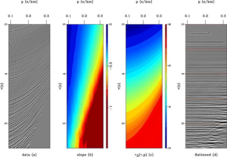
If you have sampled functions $f(x)$ and $y(x)$, sfiwarp with inv=y (the default) finds sampled $f(y)$. If inv=n, sfiwarp takes $f(y)$ and $y(x)$ and finds $f(x)$. In both cases, the sampled $y(x)$ function is supplied in a file specified by warp= parameter. The following example from milano/taupvel/cmp shows a seismic taup-p gather flattening by predictive painting and time warping.

Coordinate mapping is a fundamental data-transformation operation, which finds many applications. The term warping comes from medical imaging. See, for example,

  • Wolberg, G., 1990, Digital image warping: IEEE Computer Society Press.
  • W. Burnett and S. Fomel, 2009, Moveout analysis by time-warping: 79th Annual International Meeting, SEG, 3710-3714.

The algorithm used in sfiwarp is B-spline interpolation and inverse spline interpolation. If forward warping (inv=n) is $\mathbf{f}_x = \mathbf{B}\,\mathbf{f}_y$, then the inverse transformation (inv=y) is given by the regularized least-squares inverse
$$\mathbf{f}_y = \left(\mathbf{B}^T\,\mathbf{B} + \epsilon^2\,\mathbf{D}\right)^{-1}\,\mathbf{B}^T\,\mathbf{f}_x\;,$$ where $\mathbf{D}$ is the derivative operator. The $\epsilon$ parameter is supplied by eps=. The sampling in $y$ is supplied by n1=, d1=, o1= parameters.

For 2-D and 3-D versions, try sfiwarp2 and sfiwarp3.

10 previous programs of the month

The necessity of object orientation in geophysical software applications

August 16, 2012 Systems 3 comments

I will begin now acting on an older idea that I espoused on the blog — discussing topics of programming and software engineering related to HPC in general and Madagascar in particular. Comment feedback is more than welcome 🙂

Today’s discussion is about the necessity of light object orientation in many geophysical applications. Like medicine, object orientation can be very useful, but when used inappropriately or in large quantities can lead to severe problems. One necessity for this medicine is the case when the same algorithm applies to 2D and 3D data, with minimal changes other than adding an extra loop. Geophysicists writing code usually either create two versions of the program, or they try to only write a 3-D version that also deals with 2-D data. Creating two versions of the program leads to severe maintenance issues in the long term. The potential for bugs and forking the code is enormous. There are also other variations (anisotropy, alternative kernels, etc), so the amount of code duplication can easily explode. Writing a 3-D version that also works on 2-D data is a better option, however this usually requires contortions to introduce length-1 axes upfront in some of the inputs, and may create outputs with different dimensions for 2-D vs. 3-D, breaking workflows. The biggest block, however, comes from the fact that the 3-D code is more verbose, harder to understand and keep in mind in its entirety, and more prone to bugs. This is why people first implement a feature in the 2-D program, test it, understand it, and then upgrade the 3-D to it. Also, the simplicity of 2-D programs comes in handy when trying to explain the algorithm to other people. The way to both have the cake and eat it is through overloading (link) and light object orientation. This makes it possible to write a program that looks like a 2-D program, but also works on 3-D data. Neither C nor F90 are truly object-oriented, but they do have user-defined structures and they have static global variables that can be used to remember whether the problem is 2-D or 3-D. These features should be enough to work out a solution for this light OO problem. To convert pairs of programs that already exist as both 2D and 3D, one would first define structures that have both x and y members (i.e. offset.x and offset.y), then convert both programs to use those instead of the native types (i.e. offset_x and offset_y). Then, a test for whether the data is 2-D or 3-D is implemented, and the value preserved as a global variable so it can be accessed by various procedures without being passed as an explicit argument. Then, code sequences that have extra operations for 3D are moved into functions that are in effect overloaded, so they call a 3-D operator for 3-D data, and 2-D operator for 2-D data. In the end, the 2-D and 3-D main programs should look the same, and what is left is removing one file, renaming another, and keeping only one version.

What do you think is the best way to avoid code duplication in geophysical applications?
Program of the month: sfpick

August 1, 2012 Programs No comments

sfpick performs automatic picking from semblance-like panels.

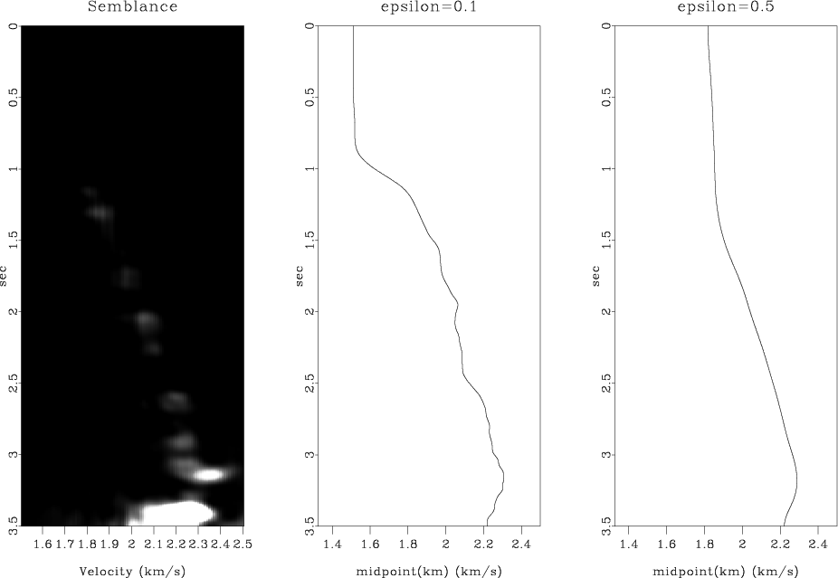
The underlying algorithm is described in Appendix B of the paper Velocity analysis using AB semblance and is inspired by the method of virtual endoscopy in medical imaging. The following example from tccs/avo/avo shows an automatic pick through AB semblance.

If smooth=n, the program picks an optimal path through the panel but does not try to smooth it. If smooth=y (the default), the picked path is additionally smoothed using shaping regularization. The smoothing radius across different dimensions is controled by rect1=, rect2=, etc. parameters. The number of shaping iterations is specified by niter=. The following example from sep/vc2/beivc shows two different picks for two different values of the rect1= parameter

The vel0= refers to the value the pick initially takes at the surface (the origin). This value is not necessarily preserved, because it can get modified by smoothing. In the following example from tccs/timelapse/timelapse, vel0=1.

The an= parameter controls the anisotropy between the two axes of the semblance panel. Varying this parameter, you can achieve picks that are more rigid or more flexible. The gate= parameter controls how far (in velocity samples) the pick can swing between two neighboring time samples. Changing its value also affects the flexibility of the picked trend.

For picking from 3-D (rather than 2-D) panels, try sfpick3.

10 previous programs of the month

FFTW

July 30, 2012 Systems No comments

FFTW (the Fastest Fourier Transform in the West) is a famous library implementing an FFT algorithm. It was developed at MIT by Matteo Frigo and Steven G. Johnson and is distributed under a GPL license.

By popular demand, Madagascar’s FFT-based programs (such as sffft1 and sffft3) include now an optional support for FFTW. The presence of the FFTW single-precision library is detected during compilation. The following table shows some peformance measurements (CPU time in seconds for 1,000 complex-valued FFTs using sffft3):

data length KISS FFT FFTW
4,096 0.11 0.08
8,192 0.27 0.18
16,384 0.50 0.32
32,768 1.21 0.80
65,536 2.61 1.78

Event of the year 2012

July 25, 2012 Celebration No comments

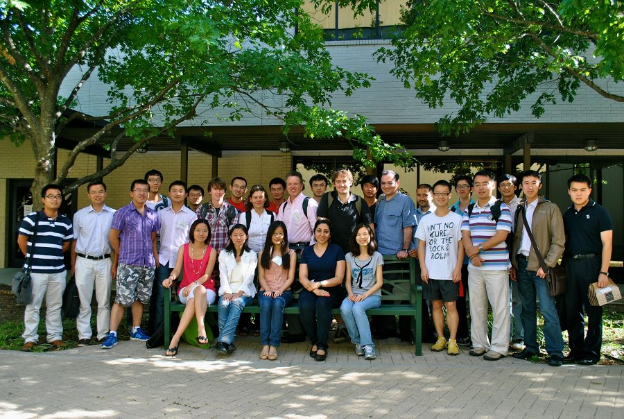
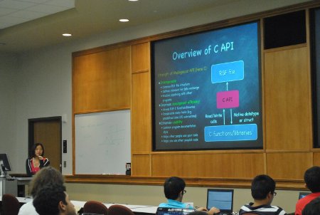
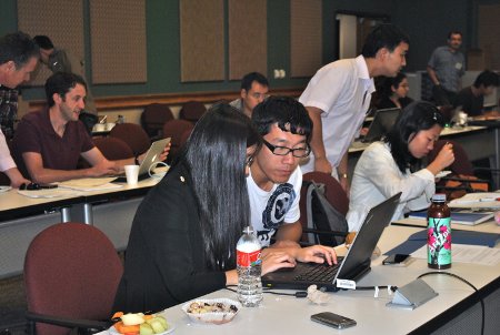
(Photos by Carla Cristina Carvajal Meneses)

The Madagascar school in Austin took place on July 20-21 and was hosted by the Bureau of Economic Geology. More than 40 people attended, representing 15 organizations (11 universities and 4 companies) from 5 different countries. The school materials are available now on the website.

Reproducible Research 2012

July 23, 2012 Links No comments

Three years after the first special issue on reproducible research, Computing in Science and Engineering published another special issue this month. The material for this issue comes from the 2011 AMP workshop Reproducible Research: Tools and Strategies for Scientific Computing organized by Randy Leveque, Ian Mitchell, and Victoria Stodden. In an editorial paper, the workshop organizers write:

The principal goal of these discussions and workshops is to develop publication standards akin to both the proof in mathematics and the deductive sciences, and the detailed descriptive protocols in the empirical sciences (the “methods” section of a paper describing the mechanics of the controlled experiment and hypothesis test). Computational science is only a few decades old and must develop similar standards, so that other researchers in the field can independently verify published results.

Program of the month: sffft3

July 2, 2012 Programs No comments

sffft3 implements a complex-to-complex Fast Fourier Transform (FFT) along an arbitrary axis.

The FFT library that Madagascar uses by default is KISS FFT, created by Mark Borgerding. KISS stands for Keep it simple, Stupid! KISS FFT may not be as fast as FFTW but it is lightweight and easy to include in the distribution.

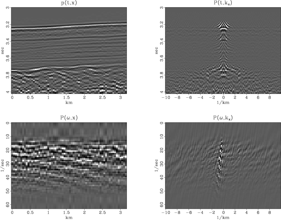
The axis= parameter specifies the data axis for performing the transform. The following example from bei/ft1/plane4 (Jon Claerbout’s Basic Earth Imaging) shows different forms of the Fourier transform applied to a 2-D dataset.

The algorithm in KISS FFT uses a mixed-radix algorithm, which is most efficient when the input size is $N=2^k\,3^l\,5^m$. By default, the input data is padded to the next optimal size, additionally multiplied by 2. To disable this behavior, use opt=n pad=1.

By default, sffft3 applies no scaling in the forward transform and $1/N$ scaling in the inverse transform. To apply a symmetric $1/\sqrt{N}$ scaling in both cases, use sym=y.

For a real-to-complex FFT along the first axis, use sffft1.

For a real-to-real Cosine Fourier Transform, use sfcosft.

To apply FFT as a linear operator, try sffft wrapper script.

10 previous programs of the month:

Why does Madagascar have such poor documentation?

June 17, 2012 FAQ No comments

Most likely, the person asking this question does not know where to look for documentation. With 6 schools, 300 blog posts, 80 wiki pages, 500-page manual and 50-page tutorial, there is plenty of information for somebody willing to learn about Madagascar or to understand how it works.

Reproducible papers and books link scientific descriptions of different algorithms with examples of their usage and thus represent the best kind of documentation scientific software may have. On the last count, there were more than 500 computational recipes (SConstruct files) and more than 5,000 reproducible figures. Reproducibility means: we provide reproducible examples of using a particular program but we do not guarantee that the program will work properly with a different choice of parameters or with different input data. With time, the ecosystem evolves. Some programs are getting used more often and, as a result, are getting better debugged and more thoroughly documented.

Madagascar has a low barrier for authors to start contributing their work. When some of the newly contributed programs and examples are not sufficiently well documented, documentation becomes a process of communication between authors and users. Engaging users as active participants in this process will help us make it more efficient.