sfcontour is a program for generating contour plots of 2-D data. It shares many of its parameters with other 2-D plotting programs, such as sfgrey and sfgraph. You can access these parameters by running sfdoc stdplot.
Let us discuss some of the parameters specific to sfcontour.
The number of contours, their origin and increment are given by nc=, c0=, dc=. If these parameters are not specified, they are determined from the data values. The contour lines in the following picture from jsg/agath/radon were created with sfcontour c0=10 dc=10 nc=10

Alternatively, the contours can be specified in a list with c= or in a file with cfile=.
By default, sfcontour plots only contours for the positive values of the input. If you want both positive and negative values to be represented, use allpos=n.
A 3-D version of sfcontour is sfcontour3.
The contour lines in the following picture from jsg/flat/comaz were created with sfcontour3 cfile=

Complex trace attributes were introduced into geophysics by the paper

Taner, M. T., F. Koehler, and R. E. Sheriff, 1979, Complex seismic trace analysis: Geophysics, 44, 1041-1063.

If $s(t)$ is the input seismic trace, then the analytical trace is defined as the complex-valued signal $a(t) = s(t)+i h(t)$, where $h(t)$ is the Hilbert transform of $s(t)$

$$h(t) =\displaystyle \frac{1}{\pi} \int \frac{s(\tau)}{t-\tau} d\tau\;.$$

The signal envelope is the positive signal $e(t)=\sqrt{s^2(t)+h^2(t)}$. A phase-rotated seismic signal is $p(t)=s(t)\,\cos{\phi} +h(t)\,\sin{\phi}$ where $\phi$ is the phase of rotation. By default, sfenvelope computes the signal envelope. It can also produce a phase-rotated signal if given hilb=y and phase=. If phase=90 (the default value), the phase-rotated signal will be simply the Hilbert transform of the input.

The following figure from book/rsf/rsf/sfenvelope illustrates an application of sfenvelope:

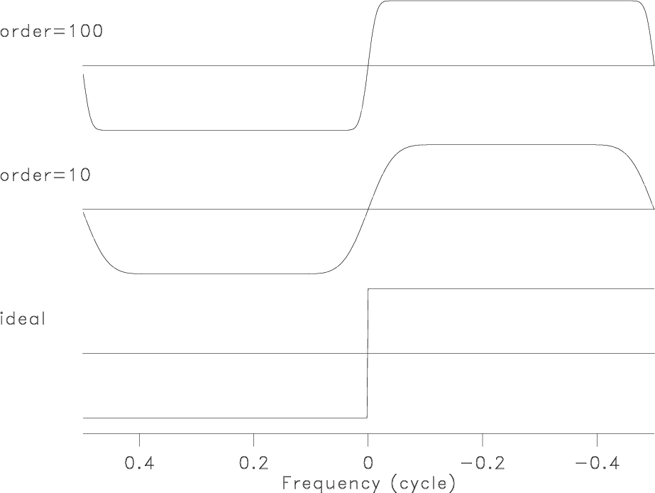
Computing the discrete Hilbert transform is not a trivial task. In the Fourier domain, the continuous Hilbert transform is given by

$$\displaystyle H(\omega) = i\,\operatorname{sgn}(\omega)\,S(\omega)$$

where $\operatorname{sgn}$ is the sign function. The discontinuity of the sign function in the frequency domain at $\omega=0$ is related to the slow $1/t$ decay of the filter impulse response in the time domain. The discontinuity at the Nyquist frequency creates additional oscillations. Different practical implementations shorten the filter impulse response by effectively smoothing the Fourier-domain discontinuities. The Madagascar implementation of the discrete Hilbert transform follows the algorithm described in

Pei, S.-C., and P.-H. Wang, 2001, Closed-form design of maximally flat FIR Hilbert transformers, differentiators, and fractional delayers by power series expansion: IEEE Trans. on Circuits and Systems, v. 48, No. 4, 389-398.

The accuracy/cost trade-off is controlled by two parameters: order= and ref=. The following figures frombook/rsf/rsf/sfenvelope illustrate the effect of the order= parameter:

The Seismic Unix implementation (suhilb program) applies a Hamming window in the time domain. For some reason, it has the filter polarity reversed:

A multidimensional analog of the Hilbert transform is the Riesz transform. It is implemented in the sfriesz program.

sfagc implements Automatic Gain Control, a popular technique for normalizing signal amplitudes.
The algorithm is simple: divide the signal by its smoothed absolute value. The smoothing is controlled by rect#= and repeat= parameters, similar to the ones used by sfsmooth.
The following example from rsf/rsf/sfagc illustrates the application of sfagc in comparison with the application of sfpow, which applies a gain based on a power of time. The gains are applied to a shot gather from Alaska from the collection of shot gathers by Yilmaz and Cumro. A similar example appears on page 236 in Jon Claerbout’s Imaging the Earth’s Interior.

For a more accurate algorithm, try sfshapeagc, which computes the gain function using shaping regularization.

sfclip is very simple yet very useful program. It “clips” the data to the specified maximum by the absolute value.

Here is a simple test. First, let us make some data.

bash$ sfmath n1=10 output="sin(x1)" > data.rsf
bash$ < data.rsf sfdisfil
   0:             0       0.8415       0.9093       0.1411      -0.7568
   5:       -0.9589      -0.2794        0.657       0.9894       0.4121

Now clip it to 0.5 by maximum absolute value.

bash$ < data.rsf sfclip clip=0.5 > clip.rsf
bash$ < clip.rsf sfdisfil
   0:           0.5          0.5          0.5       0.1411         -0.5
   5:          -0.5      -0.2794          0.5          0.5       0.4121 

What if you need to clip the data not by the maximum value but to a specified range? Use sfclip2.

bash$ < data.rsf sfclip2 lower=0 upper=0.9 > clip2.rsf
bash$ < clip2.rsf sfdisfil
   0:             0       0.8415          0.9       0.1411            0
   5:             0            0        0.657          0.9       0.4121

sfclip should handle correctly infinite values, for example those resulting from division by zero.

bash$ sfmath n1=10 output=1/x1 > data.rsf
bash$ < data.rsf sfdisfil
   0:           inf            1          0.5       0.3333         0.25
   5:           0.2       0.1667       0.1429        0.125       0.1111
bash$ < data.rsf sfclip clip=0.3 > clip.rsf
bash$ < clip.rsf sfdisfil
   0:           0.3          0.3          0.3          0.3         0.25
   5:           0.2       0.1667       0.1429        0.125       0.1111

A prototype of sfclip is used as an example in Guide to madagascar API. The actual program is a little different.

sfgraph belongs to the family of plotting programs and is used for plotting explicitly defined 2-D curves.

Here are 10 basic facts about this program:

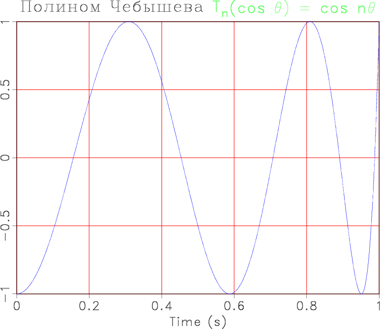
1. sfgraph shares most of its parameters with some other 2-D plotting programs (sfgrey, sfcontour, sfwiggle). These common parameters can be accessed by running sfdoc stdplot. The following plot from rsf/rsf/sfgraph is using parameters grid=y gridcol=5 pad=n and some creative changes of fonts in the title.
2. If the input to sfgraph is real, it is understood as representing a regularly sampled 1-D function Y(X), where X is sampled according to n1=, o1=, and d1= parameters in the input file.
3. If the input is complex, its real part is taken as X, and the imaginary part is taken as Y. If the input is real initially, it is easy to turn it into complex by using sfcmplx or sfdd.
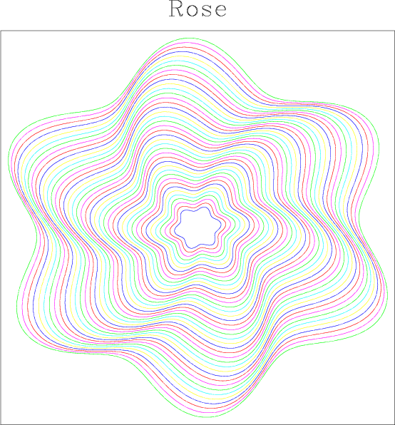
4. If the n2 parameter in the input is greater than 1, multiple curves are plotted. The following plot from rsf/rsf/sfmath shows plots of closed curves defined by a complex-valued input.
5. If the n3 or any of the larger dimensions is greater than 1, the plot becomes a movie.
6. By default, the graphs are plotted with lines. One can control the line appearance with generic parameters dash=, plotcol=, plotfat=.
   The following plot from jsg/seislet/sin2 contained dashed lines created with dash=1,2,0.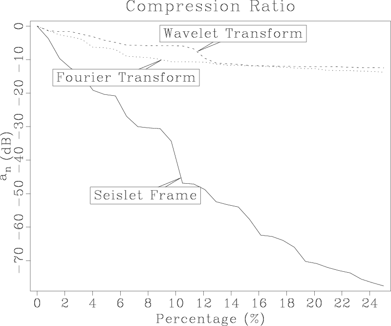
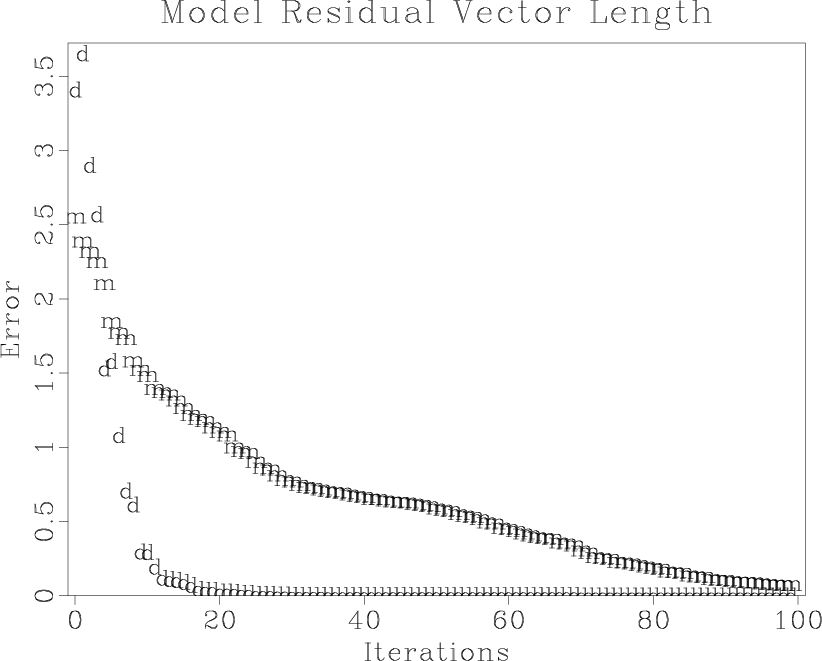
7. If symbol= is specified, the graph is plotted with the given symbols. The size of the symbol is controlled with symbolsz=. The following plot from sep/precon/oned is created with symbol=”md” symbolsz=7.
8. The displayed function can be changed from $Y(X)$ to $X(Y)$ by using transp= parameter. The following plot from jsg/nmo3/azimuthtest is created with transp=y yreverse=y symbol=+ symbolsz=4.
9. The ranges of $X$ and $Y$ are selected automatically but can be controlled with min1=, max1=, min2=, max2=.
   If you want automatic ranges, but no padding around minimum and maximum values, use pad=n.
10. sfgraph avoids plotting infinite or NaN (not a number) values.

I’m pleased today to introduce tkMadagascar, a graphical front end for Madagascar.   tkMadagascar is a very poweful, but simple way for users to create processing flows for Madagascar without needing to use the command line or a text editor.  

Here are some images of tkMadagascar in action:

Creating and configuring Flows, Plots and Results:

Viewing Madagascar program self-documentation:

Most users (>75%) will probably find that they can use tkMadagascar solely in place of command line tools and/or text editors.  However, power users will likely find that it is somewhat limiting (e.g. no Python command support).  

You can dive into tkMadagascar if you are using the development version by updating, and reinstalling Madagascar.  

Additional documentation and tutorials can be found here.

Vladimir Bashkardin contributes a Vplot plugin for PLplot, an open-source scientific plotting library. Here is an example of generating Vplot files with PLplot using sfplsurf.

A previous entry ranked most popular Madagascar programs by the number of projects they are used in. A different approach to ranking is to use network analysis algorithms. If we declare that the two programs are linked if they are used in the same project, then all links define a network, and we can use the PageRank algorithm devised by Google to find the largest “hubs” in the network. Similarly, two projects are linked if the use the same program, which defines a network and ranking among projects. The admin/rank.py script does the job. In reverse order, the 10 top ranked programs in Madagascar are:

10. sftransp Transpose two axes in a dataset.

9. sfput Input parameters into a header.

8. sfgraph Graph plot.

7. sfcat Concatenate datasets.

6. sfspike Generate simple data: spikes, boxes, planes, constants.

5. sfadd Add, multiply, or divide RSF datasets.

4.sfdd Convert between different formats.

3.sfmath Mathematical operations on data files.

2.sfwindow Window a portion of a dataset.

1.sfgrey Generate raster plot.

More documentation on these and other programs – in Guide to Madagascar programs. The three top ranked programs in the “generic” category (signal processing programs applicable to any kind of data) are smooth (Multi-dimensional triangle smoothing), sfnoise (Add random noise to the data), and sfbandpass (Bandpass filtering). The three top ranked programs in the “seismic” category (signal processing programs applicable to seismic data) are sfricker1 (Convolution with a Ricker wavelet), sfmutter (Muting), and sfsegyread (Convert a SEG-Y or SU dataset to RSF).

The following projects share the top rank in terms of being hubs for programs:

• bei/vela/vscan
• cwp/geo2007StereographicImagingCondition/flat4
• cwp/geo2007StereographicImagingCondition/gaus1
• cwp/geo2007StereographicImagingCondition/sigsbee2
• cwp/geo2008InterferometricImagingCondition/circle
• cwp/geo2008InterferometricImagingCondition/sact1
• cwp/geo2008NumericWEMVAoperators/flatWEMVA
• cwp/geo2008NumericWEMVAoperators/saltWEMVA
• cwp/jse2006RWEImagingOverturningReflections/sigsbee
• data/amoco/fdmod
• data/marmousi/fdmod
• data/pluto/fdmod
• data/sigsbee/fdmod2A
• data/sigsbee/ptest
• gpgn658/fdmod/exercise
• gpgn658/rtmig/exercise
• jsg/atten/enerd
• jsg/attr/vecta
• jsg/nmo3/azimuthtest
• rsf/rsf/sfawefd
• rsf/school/complex
• rsf/school/sigsbee
• rsf/school/single
• sep/burg/gtens
• sep/fmeiko/tri
• sep/precon/cube
• sep/stoltst/imps

oglpen is a new “pen” contributed by Vladimir Bashkardin. It displays Vplot files using OpenGL and GLUT and can serve as a replacement for xtpen.

vpconvert is a script for converting Vplot files to other formats (EPS, PS, PDF, PPM, TIFF, JPEG, PNG, GIF, MPEG, AVI, SVG). You can use it for converting one file

bash$ vpconvert file.vpl file.jpg

or a collection of files

bash$ vpconvert format=tiff Fig/*.vpl

Meet gdpen, a new “pen” program. gdpen converts vplot files to PNG or JPEG, or GIF graphics formats (including animated GIFs). Use it like this:

gdpen < file.vpl > file.png

or

gdpen type=jpeg < file.vpl > file.jpg

or

gdpen type=gif < file.vpl > file.gif

Other usual options are available.
gdpen requires the GD library at the compilation time.
Several other “pens” are under development:

• cairopen – for outputting standard vector-graphics formats
• svgpen – for outputting SVG directly
• pdfpen – for outputting PDF directly
• gtkpen/oglpen – for displaying plots on a screen (as a replacement for xtpen)