A new paper is added to the collection of reproducible documents: Signal and noise separation in prestack seismic data using velocity-dependent seislet transform
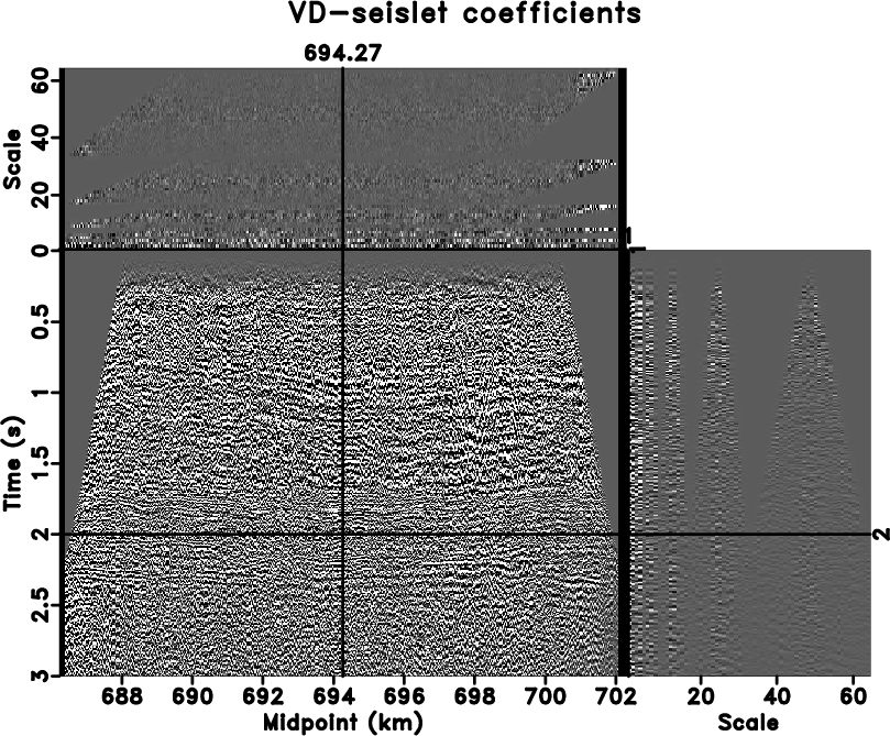
The seislet transform is a wavelet-like transform that analyzes seismic data by following varying slopes of seismic events across different scales and provides a multiscale orthogonal basis for seismic data. It generalizes the discrete wavelet transform (DWT) in the sense that DWT in the lateral direction is simply the seislet transform with a zero slope. Our earlier work used plane-wave destruction (PWD) to estimate smoothly varying slopes. However, PWD operator can be sensitive to strong noise interference, which makes the seislet transform based on PWD (PWD-seislet transform) occasionally fail in providing a sparse multiscale representation for seismic field data. We adopt a new velocity-dependent (VD) formulation of the seislet transform, where the normal moveout equation serves as a bridge between local slope patterns and conventional moveout parameters in the common-midpoint (CMP) domain. The velocity-dependent (VD) slope has better resistance to strong random noise, which indicates the potential of VD seislets for random noise attenuation under 1D earth assumption. Different slope patterns for primaries and multiples further enable a VD-seislet frame to separate primaries from multiples when the velocity models of primaries and multiples are well disjoint. Results of applying the method to synthetic and field-data examples demonstrate that the VD-seislet transform can help in eliminating strong random noise. Synthetic and field-data tests also show the effectiveness of the VD-seislet frame for separation of primaries and pegleg multiples of different orders.

