Program of the month: sfstolt

August 3, 2014 Programs No comments

sfstolt implements zero-offset (post-stack) seismic migration using Stolt method.

Stolt migration is described in the classic paper

Stolt, R. H., 1978, Migration by Fourier transform: Geophysics, 43, 23-48.

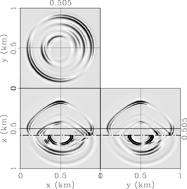
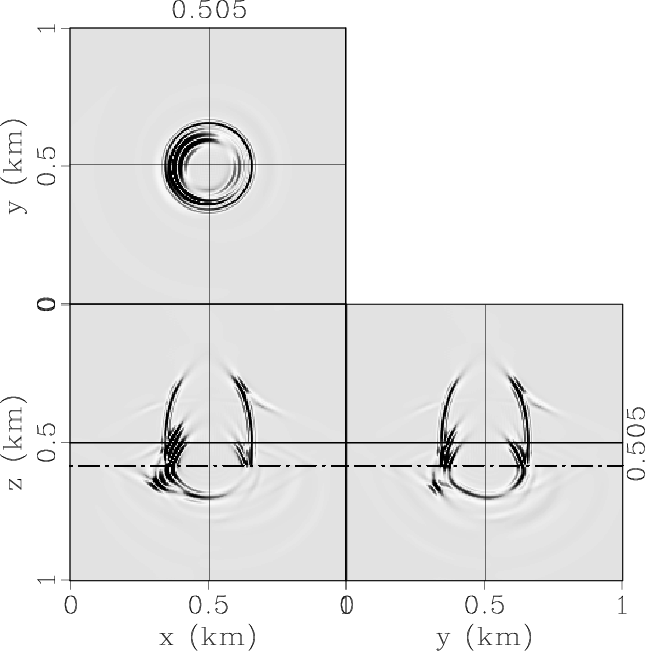
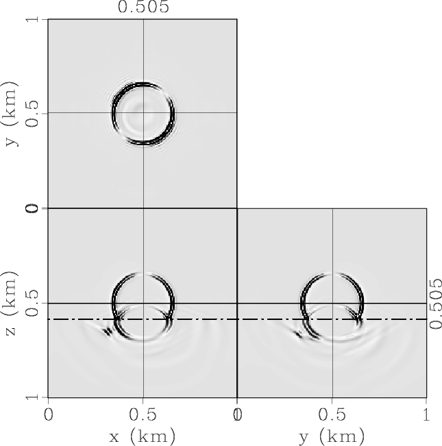
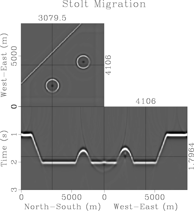
The following example from gallery/french/stolt shows the result of Stolt migration in the French model:

The classic Stolt migration works for constant velocity. However, it can be extended to the case of V(z) by using Stolt stretch and cascaded migrations. See Evaluating the Stolt-stretch parameter and its references, including

Beasley, C., W. Lynn, K. Larner, and H. Nguyen, 1988, Cascaded frequency-wavenumber migration – Removing the restrictions on depth-varying velocity: Geophysics, 53, 881-893.

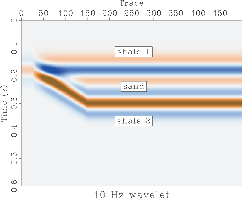
The following example from sep/stoltst/elfst compares the results of Stolt migration with Stolt stretch, phase-shift migration, and cascaded Stolt migration with Stolt stretch.

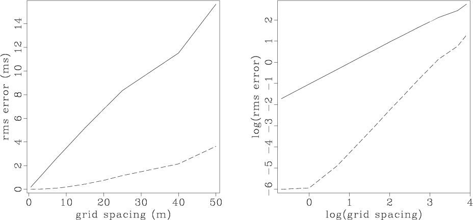
sfstolt2 is another version of Stolt migration, with a control on interpolation accuracy. The following example from sep/forwd/stolt compares results from two different interpolations:

10 previous programs of the month:

Program of the month: sfltft

July 13, 2014 Programs No comments

sfltft (Local Time-Frequency Transform) decomposes input data into frequency components.

The algorithm is described in the paper Seismic data analysis using local time-frequency decomposition and is based on regularized non-stationary regression. The following example from tccs/ltft/timefreq shows 1-D synthetic data composed of two chirp signals and the magnitude of coefficients in its time-frequency decomposition:

The frequency sampling in the output of sfltft is controled by nw=, w0=, and dw=. By default, these parameters correspond to the sampling of the discrete Fourier transform. The critical parameters for regularized regression are rect= (smoothing radius in time, in samples) and niter= (number of iterations). To output the details of iterative regularization, use verb=y. The frequency sampling and the rect= parameter provide explicit controls on time-frequency resolution. In the example above, rect=7. It is possible to change smoothing radius with frequency by using alpha= parameter. The iterative inversion can be controlled additionally by specifying a data weight (with mask=) or a model weight (with weight=). Optionally, the Fourier basis used in the decomposition can be extracted from the program by specifying basis= file.

To perform the inverse transform from time-frequency back to time domain, use inv=y. sfltft takes real-valued input and produces complex-valued output.

An analogous program for transforming complex-valued data is sfcltft. A related program is sftimefreq described in Time-frequency analysis of seismic data using local attributes.

10 previous programs of the month:

Madagascar in the cloud

July 10, 2014 Systems No comments

SageMathCloud is a free cloud computing platform for computational mathematics created by William Stein, the leader of the Sage project.

SageMathCloud provides a rich environment, which allows one, for example, to easily install Madagascar and to access it interactively through its Python interface. The example above shows Madagascar running interactively in the cloud using an IPython notebook hosted by SageMathCloud. Support for interactive widgets is a new feature in IPython version 2 released earlier this year.

See also:

Making a wedge

July 1, 2014 Examples No comments

The example in rsf/tutorials/wedge reproduces the example from Evan Bianco of simple convolution modeling with a wedge model.

See also:

Fast elastic mode separation in anisotropic media

June 24, 2014 Documentation No comments

A new paper is added to the collection of reproducible documents:
Fast algorithms for elastic-wave-mode separation and vector decomposition using low-rank approximation for anisotropic media

Wave mode separation and vector decomposition are significantly more expensive than wavefield extrapolation and are the computational bottleneck for elastic reverse-time migration (ERTM) in heterogeneous anisotropic media. We express elastic wave mode separation and vector decomposition for anisotropic media as space-wavenumber-domain operations in the form of Fourier integral operators, and develop fast algorithms for their implementation using their low-rank approximations. Synthetic data generated from 2D and 3D models demonstrate that these methods are accurate and efficient.

How do I do interactive picking?

June 12, 2014 FAQ No comments

While interactive picking is generally discouraged because of its non-reproducibility, occasionally it might be useful. Using interact= option with xtpen outputs mouse-click coordinates in a text file. However, they are Vplot coordinates, not easily related to physical coordinates of the image. Joe Dellinger has a more comprehensive plan for adding interactivity to Vplot graphics.

sfipick is a simple Tkinter script which allows for interactive picking. The interface is straightforward. Use left-button mouse clicks to add picks, right-button mouse clicks to remove wrong picks, middle-button to drag picks. The picks are written in a plain text file and can be processed later.

See also:

Program of the month: sfeikonal

June 11, 2014 Programs No comments

sfeikonal solves the eikonal equation using the Fast Marching Method. This computation produces first-arrival traveltimes on a fixed grid.

The following example from sep/fmeiko/fmarch shows traveltime contours for a point source inside the SEG/EAGE salt model.

The point source can be specified by its coordinates xshot=, yzhot=, and zshot= (note that the depth coordinate zshot corresponds to the first axis). In a small box around the source, the solution is computed analytically to avoid errors from the point-source singularity. The size of the box can be specified in samples (b1=, b2=, and b3=) or in physical dimensions (br1=, br2=, and br3=). For a plane-wave source instead of a point source, use plane1=y, plane2=y, or plane3=y. The plane is assumed to be aligned with the grid. For computing a traveltime table with multiple sources, the source coordinates can be specified in a file given by shotfile=. The order of accuracy in the finite-difference scheme is specified by order= parameter.

The following plot from sep/fmsec/cvel shows the error difference between the first- and second-order computations in a constant-velocity medium.

sfeikonal computes isotropic traveltimes. For an extension to VTI anisotropy, see sfeikonalvti.

10 previous programs of the month:

Lowrank on a staggered grid

June 2, 2014 Documentation No comments

A new paper is added to the collection of reproducible documents:
Lowrank seismic wave extrapolation on a staggered grid

We propose a new spectral method and a new finite-difference method for seismic wave extrapolation in time. Using staggered temporal and spatial grids, we derive a wave extrapolation operator using a lowrank decomposition for a first-order system of wave equations and design the corresponding finite-difference scheme. The proposed methods extend previously proposed lowrank and lowrank finite-difference wave extrapolation methods from the cases of constant density to those of variable density. Dispersion analysis demonstrates that the proposed methods have high accuracy for a wide wavenumber range and significantly reduce the numerical dispersion. The method of manufactured solutions coupled with mesh refinement is used to verify each method and to compare numerical errors. 2-D synthetic examples demonstrate that the proposed method is highly accurate and stable. The proposed methods can be used for seismic modeling or reverse time migration.

Second working workshop

June 1, 2014 Celebration 2 comments

Registration is open for Madagascar’s Second Working Workshop.

As a reminder, Working Workshops as opposed to “talking workshops” are meetings where the participants work together (possibly divided into pairs or small teams) to develop new software code or to conduct computational experiments addressing a particular problem. The First Working Workshop took place last summer in Austin. This year’s workshop will take place on at Rice University in Houston, Texas, on July 31 – August 2, 2014. The topic of this year’s workshop is parallel and high-performance computing. The objective is

  1. To develop convenient tools for high-performance and parallel computing.
  2. To create new examples of distributed-memory and shared-memory parallel computing.
  3. To explore hardware-accelerated parallel computing (NVIDIA GPU and Intel® Xeon Phi™).

Registration is free by an application is required. If you are interested in participating in this workshop, please fill an application form.

Tutorial on wave propagation

May 30, 2014 Documentation No comments

A new paper is added to the collection of reproducible documents:
Pengliang Yang from Xi’an Jiaotong University contributes A numerical tour of wave propagation

This tutorial is written for beginners as an introduction to basic wave propagation using finite difference method, from acoustic and elastic wave modeling, to reverse time migration and full waveform inversion. Most of the theoretical delineations summarized in this tutorial have been implemented in Madagascar with Matlab, C and CUDA programming, which will benefit readers’ further study.