Programs

Program of the month: sfcostaper

April 2, 2014 Programs No comments

sfcostaper applies cosine tapering to the edges of the input data.

Cosine tapering amounts to multiplying the edges by
$$\sin^2\left(\frac{\pi\,x}{2}\right) = \frac{1+\cos{(\pi\,x)}}{2}$$,
where $x$ is the relative distance from the start of the taper.

sfcostaper works in N dimensions, the size of the taper in #th dimension in samples is specified by nw#=. In the following example from gee/ajt/igrad1 the images are tapered at both edges by specifying nw1=50 nw2=50.

10 previous programs of the month:

Program of the month: sflpad

March 11, 2014 Programs No comments

sflpad pads the input data by inserting zero traces and zero planes between traces and planes in the input. The following example from gee/lal/lace shows a classic example of interpolation beyond aliasing, which appears on the cover of Jon Claerbout’s book Processing Versus Inversion:

10 previous programs of the month:

Program of the month: sfdipfilter

February 6, 2014 Programs No comments

sfdipfilter filters input data based on a range of dips (slopes).

The following example from rsf/su/rsfdipfilt (borrowed from one of Seismic Unix demos) shows a synthetic dataset with three events before and after dip filtering:

sfdipfilter operates in 2-D or 3-D Fourier transform domain, with the dimensionality specified by dim=. The dip range is specified either by angles (if angle=y) or by velocities (if angle=n). The four parameters (either ang1=, ang2=, ang3=, ang4= or v1=, v2=, v3=, v4=) specify the range. If pass=y, the range between v2 and v3 is passed, and the range below v1 or above v4 is rejected. If pass=n, the range between v2 and v3 is rejected, and the range below v1 or above v4 is passed. The transition between pass and reject regions is implemented with a sine tapering.

10 previous programs of the month

Program of the month: sfinttest1

January 9, 2014 Programs No comments

sfinttest1 performs forward interpolation from a regular grid to irregular locations (in 1-D).

The following example from sep/forwd/chirp shows regularly sampled values of a variable-frequency signal and the error of its interpolation using linear and cubic-convolution interpolators.

The irregular coordinates for interpolation are supplied in a file specified by coord=. The type of the interpolator is specified by interp=. The currently implemented types are Lagrange (including linear and nearest-neighbor interpolation), cubic convolution, weighted sinc interpolation (with Kaiser, Lanczos, cosine, and Welsh windows), B-spline, and MOM (slightly improved B-spline). The size of the interpolation filter is given by nw=. The Kaiser-window interpolator requires an additional parameter, which is specified by kai=.

An alternative (using invertible cubic spline interpolation) is sfiwarp.

A 2-D version is sfinttest2. The following example from sep/forwd/chirp2 compares the error of Kaiser-windowed 8-point sinc interpolation and 8-point B-spline interpolator applied to interpolating a 2-D signal.

10 previous programs of the month

Program of the month: sfcausint

December 1, 2013 Programs No comments

sfcausint implements an operation of causal numerical integration. This is a simple operation, which mathematically amounts to recursion
$$yn = y{n-1} + x_n$$
or to inversion of a simple bidiagonal matrix. See Geophysical Image Estimation by Example for more explanation.

The only parameter in sfcausint is adj=, the flag for adjoint computation. The adjoint operation applies recursion backwards
$$x{n-1} = xn + y_{n-1}$$

The following example from gee/ajt/causint illustrates forward and ajoint causal integration with sfcausint:

10 previous programs of the month

Program of the month: sfremap1

November 3, 2013 Programs No comments

sfremap1 interpolates the input data to a different grid along the first axis. Here is an elementary example: making some data and interpolating it to a denser grid:

bash$ sfmath n1=5 o1=0 d1=1 output=x1 | sfdisfil 
0: 0 1 2 3 4 
bash$ sfmath n1=5 o1=0 d1=1 output=x1 | sfremap1 n1=10 d1=0.5 | sfdisfil 
0: 0 0.5 1 1.5 2 
5: 2.5 3 3.5 4 4.5

sfremap1 uses ENO (essentially non-oscillatory) interpolation to prevent oscillations when interpolating discontinuous data:

bash$ sergey$ sfspike n1=10 o1=0 d1=1 k1=6 | sfcausint | sfdisfil 
0: 0 0 0 0 0 
5: 1 1 1 1 1 
bash$ sfspike n1=10 o1=0 d1=1 k1=6 | sfcausint | sfremap1 n1=20 d1=0.5 | sfdisfil 
0: 0 0 0 0 0 
5: 0 0 0 0 0.5 
10: 1 1 1 1 1 
15: 1 1 1 1 1

The ENO algorithm is described by Harten et al. (1987) and Shu and Osher (1988):

A. Harten, B. Engquist, S. Osher, and S. R. Chakravarthy, 1987, Uniformly high order accurate essentially non-oscillatory schemes, III: Journal of Computational Physics, 71(2), 231-303.

C. W. Shu and S. Osher, 1988, Efficient implementation of essentially non-oscillatory shock-capturing schemes: Journal of Computational Physics, 77(2), 439-471.

The interpolation order is controlled by the order= parameter, order=2 corresponds to linear interpolation, the default is order=3. The output grid can be specified either by n1=, o1=, d1= parameters or by providing an example file with the desired grid in pattern= parameter. Here is an example:

bash$ sfmath n1=5 o1=0 d1=1 output=x1 > data.rsf
bash$ sfspike n1=10 d1=0.5 > other.rsf
bash$ < data.rsf sfremap1 pattern=other.rsf | sfdisfil
   0:             0          0.5            1          1.5            2
   5:           2.5            3          3.5            4          4.5

For an alternative method (cubic spline interpolation), see sfspline.

10 previous programs of the month:

Program of the month: sfunif2

October 3, 2013 Programs No comments

sfunif2 creates a layered model from specified interfaces. It is inspired by an analogous program in Seismic Unix.

The following example from rsf/su/rsfmodel shows a simple model generated with sfunif2 and reproduced from an example in the book Seismic Data Processing with Seismic Un*x by David Forel, Thomas Benz, and Wayne Pennington.

The input to sfunif2 is a file containing sampled interfaces. The velocities in the layers can be specified as linear distributions
$$v(z,x) = v_0 + v_z\,(z-z_0)+v_x\,(x-x_0)$$
with parameters given by v00=, dvdz=, dvdx=, z0=, and x0=. These parameters should be lists, with the number of elements greater by one than the number of interfaces. The desired sampling of the depth axis is specified by n1=, o1=, and d1= parameters.

The 3-D version is sfunif3. See the following example from rsf/rsf/unif3

In addition to specifying layer velocities as linear (constant gradient) distributions, sfunif3 allows these properties to be specified in an optional file.

10 previous programs of the month

Program of the month: sfpatch

September 14, 2013 Programs No comments

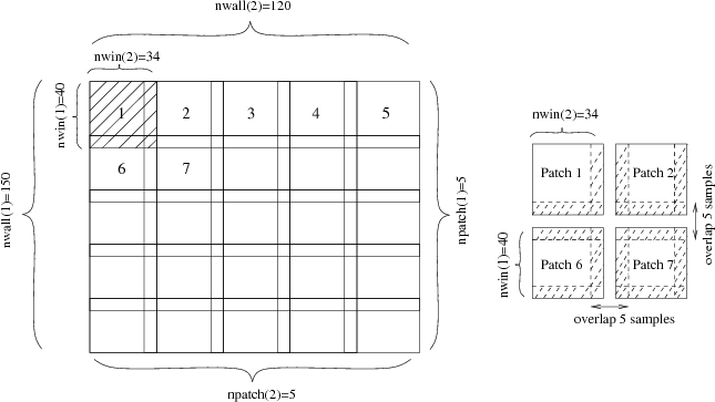
sfpatch breaks the input data into local windows or “patches”, possibly with overlap.

The patching technique is explained by Jon Claerbout in Nonstationarity: patching chapter from Image Estimation by Example.

Suppose you have a 1-D signal with 10 samples:

bash$ sfmath n1=10 output=x1 > data.rsf

You can divide it, for example, into two patches with 5 samples each:

bash$ < data.rsf sfpatch p=2 w=5 > patch.rsf
bash$ sfget n1 n2 < patch.rsf 
n1=5
n2=2

or into 5 overlapping patches with 3 samples each:

bash$ < data.rsf sfpatch p=5 w=3 > patch.rsf
bash$ sfget n1 n2 < patch.rsf 
n1=3
n2=5

If you specify only the patch size (w= parameter), sfpatch tries to select the number of patches to achieve a good overlap:

bash$ < data.rsf sfpatch w=3 > patch.rsf
bash$ sfget n1 n2 < patch.rsf 
n1=3
n2=6

If you put overlapped patches back together, their amplitudes add in the overlapped regions:

bash$ < data.rsf sfdd type=int | sfdisfil 
   0:    0    1    2    3    4    5    6    7    8    9
bash$< patch.rsf sfpatch inv=y | sfdd type=int | sfdisfil
   0:    0    2    6    6    8   10   12   14    8    9

unless you use the weight option:

bash$ < patch.rsf sfpatch inv=y weight=y | sfdd type=int | sfdisfil
   0:    0    1    2    3    4    5    6    7    8    9

bash$ sfpatch easily handles multidimensional data: w= and p= become lists of dimensions, and the number of dimensions in the output effectively doubles. sfpatch is useful in two applications:

  1. crude handling of non-stationarity when processing non-stationary signals with locally stationary filters,
  2. making non-parallel tasks data-parallel.

A simple example from rsf/rsf/mona illustrates the second use.

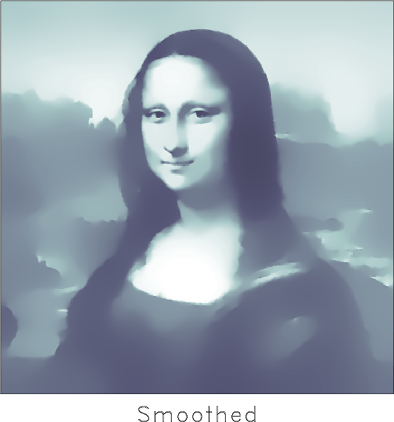
Anisotropic diffusion, implemented by sfimpl2, is an effective but relatively slow process. By breaking the input 512×512 image into nine 200×200 overlapping patches and by processing them in parallel on a multi-core computer, we can achieve a significant speed-up without rewriting the original program.

10 previous programs of the month

Telling your story with sfresults

September 11, 2013 Programs No comments

Sometimes it is convenient to have a quick access to all results in your experiment. sfresults, a simple Tkinter script, provides that functionality. Run this script in your project directory. Click on “Cycle” button to run scons view, click on an individual result button to run scons result.view, or select several results and click on “Flip” to flip between the figures on the screen.

Program of the month: sfai2refl

August 2, 2013 Programs No comments

sfai2refl converts acoustic impedance to normal-incidence PP reflectivity using the simple equation
$$R(t) = \frac{I(t+\Delta t) – I(t)}{I(t+\Delta t) + I(t)}$$

The program is useful for convolution modeling. The following example from rsf/rsf/wedge shows a classic example of wedge modeling, which is used for analyzing the tuning phenomenon (Kallweit, R. and L. Wood, 1982, The limits of resolution of zero-phase wavelets: Geophysics, v. 47, 1035–-1046.)

A more sophisticated example from geo384w/hw5/sigsbee2 computes an effective reflectivity of the Sigsbee model:

The program has no parameters.

10 previous programs of the month