Just for fun… sfmandelbrot computes the famous Mandelbrot set. See examples in rsf/rsf/fractal.

Zooming in, one can explore different fractal patterns inside the set.

More fractal fun
September 24, 2006 Examples No comments
Fractals
July 11, 2006 Examples No comments
Just for fun… sffern computes “fractal ferns”. See an example in rsf/rsf/fractal and an animated gif.

Checking parameters
July 10, 2006 Examples No comments
It its now possible to check parameters for Madagascar programs in SCons flows using CHECKPAR option like this: scons CHECKPAR=y <target> Here is what happened when I first ran an example from rsftour:
bash$ scons CHECKPAR=y
scons: Reading SConscript files ...
No parameter "n2" in sfwindow
Failed on "window n2=10 min1=0.4 max1=0.8"
After fixing self-documentation for sfwindow:
bash$ scons CHECKPAR=y
scons: Reading SConscript files ...
No parameter "nc" in sfwiggle
Failed on "wiggle transp=y poly=y yreverse=y pclip=100 nc=100 allpos=n "
Fixing that one requires changing the SConstruct file.
CHECKPAR is an experimental option and will be enhanced in the future to include parameter ranges and other safety checks. Another useful option is TIMER.
Timing the execution
June 3, 2005 Examples No comments
You can now time the execution of processing flows in Scons using a TIMER option. Use it like this:
scons TIMER=y <target>
An example from rsftour:
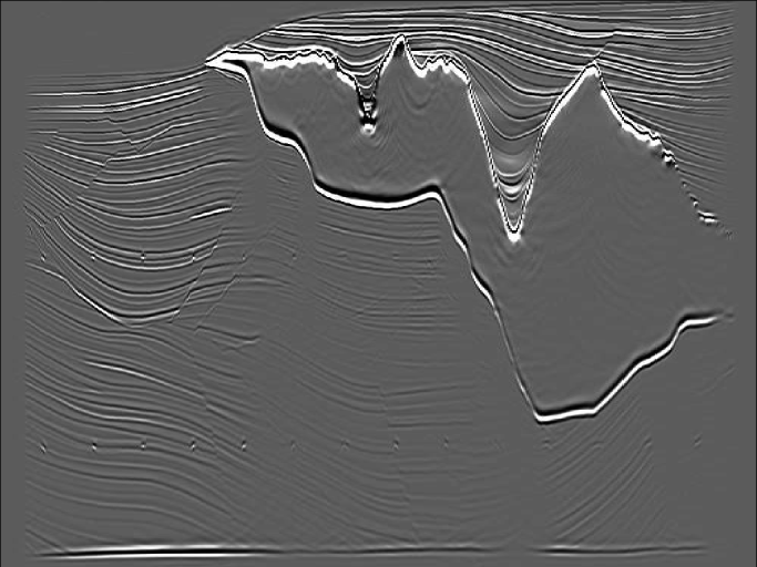
Wave equation prestack depth migration
April 23, 2005 Examples No comments
Here is Paul Sava’s result on imaging Sigsbee2A synthetic dataset using wave equation migration on a cluster.
Stochastic simulation
March 29, 2005 Examples No comments
In pbi/modl/random, Jim Jennings creates an example of random correlated field with exponential covariance.

Ray tracing
March 24, 2005 Examples No comments
Some examples of ray tracing with sfrays2 are in gti/timec/paul. See also sfcell2 and sfshoot2.

Finite-differences modeling
March 23, 2005 Examples No comments
Here is a time-domain finite-difference example in RSF.
The program allows arbitrary locations of the sources and receivers.
The following pictures are examples using the Marmousi model.
The sources are located on a horizontal line close to the bottom of the model.
The receivers are arranged as in a deviated well.
Velocity:

Wavefield snapshot:

Recorded data:
