Month: April 2014

IWAVE update

April 28, 2014 Documentation No comments

The IWAVE package included in Madagascar went through a significant redesign. The current version is explained in the paper IWAVE Structure and Basic Use Cases by Bill Symes.

The IWAVE control structure facilitates construction of wave simulators with flexible specification of input and output. This document describes synthesis of seismograms and wavefield movies from initial data and from single and multiple sources (right-hand sides), and linearized (“Born”) and linearized adjoint (reverse time migration) modeling. The choice of physical model and simulation method – constant density acoustics with Dirichlet boundary conditions and (2,2k) finite difference schemes – is the simplest possible, but the framework accommodates any regularly gridded stencil-based discretization of arbitrary wave physics in the same way.

GPU implementation of RTM

April 26, 2014 Documentation No comments

A new paper is added to the collection of reproducible documents:
RTM using effective boundary saving: A staggered grid GPU implementation

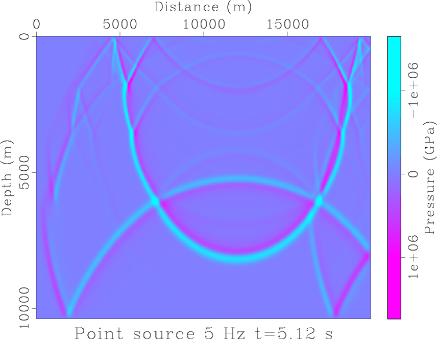
GPU has become a booming technology in reverse time migration (RTM) to perform the intensive computation. Compared with saving forward modeled wavefield on the disk, RTM via wavefield reconstruction using saved boundaries on device is a more efficient method because computation is much faster than CPU-GPU data transfer. In this paper, we introduce the effective boundary saving strategy in backward reconstruction for RTM. The minimum storage requirement for regular and staggered grid finite difference is determined for perfect reconstruction of the source wavefield. Particularly, we implement RTM using GPU programming, combining staggered finite difference scheme with convolutional perfectly matched layer (CPML) boundary condition. We demonstrate the validity of the proposed approach and CUDA codes with numerical example and imaging of benchmark models.

This paper is the first contribution from Xi’an Jiaotong University in China.

Random noise attenuation by EMD predictive filtering

April 23, 2014 Documentation No comments

A new paper is added to the collection of reproducible documents:
Random noise attenuation by f-x empirical mode decomposition predictive filtering

Random noise attenuation always plays an important role in seismic data processing. One of the most widely used methods for suppressing random noise is f-x predictive filtering. When the subsurface structure becomes complex, this method suffers from higher prediction errors owing to the large number of different dip components that need to be predicted. In this paper, we propose a novel denoising method termed f-x empirical mode decomposition predictive filtering (EMDPF). This new scheme solves the problem that makes f-x empirical mode decomposition (EMD) ineffective with complex seismic data. Also, by making the prediction more precise, the new scheme removes the limitation of conventional f-x predictive filtering when dealing with multi-dip seismic profiles. In this new method, we first apply EMD to each frequency slice in the f-x domain and obtain several intrinsic mode functions (IMF). Then an auto-regressive (AR) model is applied to the sum of the first few IMFs, which contain the high-dip-angle components, in order to predict the useful steeper events. Finally, the predicted events are added to the sum of the remaining IMFs. This process improves the prediction precision by utilizing an EMD based dip filter to reduce the dip components before f-x predictive filtering. Both synthetic and real data sets demonstrate the performance of our proposed method in preserving more useful energy.

Pseudo-pure wave modes in anisotropic media

April 20, 2014 Documentation No comments

A new paper is added to the collection of reproducible documents:
Simulating propagation of separated wave modes in general anisotropic media, Part I: qP-wave propagators
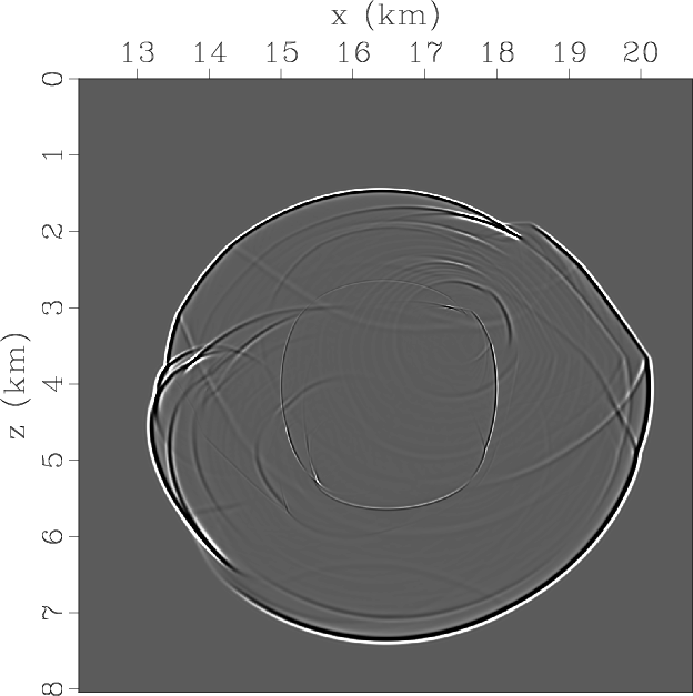
Wave propagation in an anisotropic medium is inherently described by elastic wave equations, with P- and S-wave modes intrinsically coupled. We present an approach to simulate propagation of separated wave modes for forward modeling, migration, waveform inversion and other applications in general anisotropic media. The proposed approach consists of two cascaded computational steps. First, we simulate equivalent elastic anisotropic wavefields with a minimal second-order coupled system (that we call here a pseudo-pure-mode wave equation), which describes propagation of all wave modes with a partial wave mode separation. Such a system for qP-wave is derived from the inverse Fourier transform of the Christoffel equation after a similarity transformation, which aims to project the original vector displacement wavefields onto isotropic references of the polarization directions of qP-waves. It accurately describes the kinematics of all wave modes and enhances qP-waves when the pseudo-pure-mode wavefield components are summed. The second step is a filtering to further project the pseudo-pure-mode wavefields onto the polarization directions of qP-waves so that residual qS-wave energy is removed and scalar qP-wave fields are accurately separated at each time step during wavefield extrapolation. As demonstrated in the numerical examples, pseudo-pure-mode wave equation plus correction of projection deviation provides a robust and flexible tool for simulating propagation of separated wave modes in transversely isotropic and orthorhombic media. The synthetic example of Hess VTI model shows that the pseudo-pure-mode qP-wave equation can be used in prestack reverse-time migration (RTM) applications.

This paper is the first contribution from Tongji University in Shanghai, China.
Program of the month: sfcostaper

April 2, 2014 Programs No comments

sfcostaper applies cosine tapering to the edges of the input data.

Cosine tapering amounts to multiplying the edges by
$$\sin^2\left(\frac{\pi\,x}{2}\right) = \frac{1+\cos{(\pi\,x)}}{2}$$,
where $x$ is the relative distance from the start of the taper.

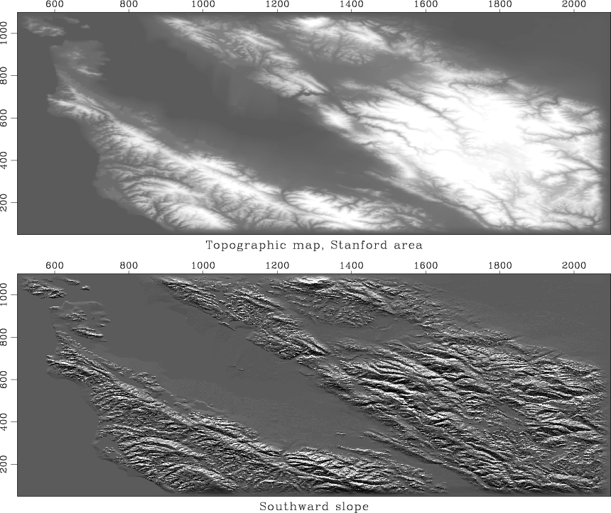
sfcostaper works in N dimensions, the size of the taper in #th dimension in samples is specified by nw#=. In the following example from gee/ajt/igrad1 the images are tapered at both edges by specifying nw1=50 nw2=50.

10 previous programs of the month: