A new paper is added to the collection of reproducible documents:
Modeling of pseudo-acoustic P-waves in orthorhombic media with a lowrank approximation
Lowrank modeling in orthorhombic media
June 25, 2013 Documentation No comments
Kirchhoff migration with traveltime source-derivatives
June 24, 2013 Documentation No comments
A new paper is added to the collection of reproducible documents:
Kirchhoff migration using eikonal-based computation of traveltime source-derivatives

Extending MATLAB interface
June 13, 2013 Systems No comments
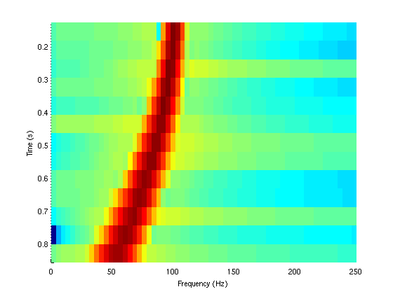
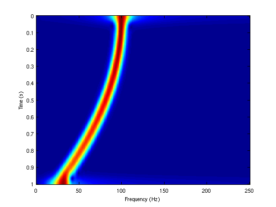
For those using MATLAB interface to Madagascar, a new function, m8r, allows running Madagascar programs and workflows directly on MATLAB objects. The following MATLAB code runs regularized time-frequency analysis using sftimefreq:
% create chirp signal
t=0:0.001:1;
y=chirp(t,100,1,25,'q',[],'convex');

% spectragram analysis in MATLAB
spectrogram(y,256,200,256,1000);
set(gca,'xlim',[0,250]);
set(gca,'ydir','reverse');
ylabel('Time (s)');
% time-frequency analysis in Madagascar
tf = m8r('sftimefreq rect=50 nw=251 dw=1',y',0.001);

f = 0:250;
imagesc(t,f,tf);
xlabel('Frequency (Hz)');
ylabel('Time (s)');
Program of the month: sfwiggle
June 12, 2013 Programs No comments
sfwiggle plots data using the traditional seismic method of wiggly traces.
The following example from rsf/rsf/rsftour shows a typical output:
Similarly to other plotting programs, there are multiple parameters that control the output. For example, poly=y draws solid polygons for highlighting positive data, transp=y transposes the two axes, xreverse=y or yreverse=y reverse the corresponding axis. Data scaling is controlled with either the absolute clip (clip=) or percentage clip (pclip=).
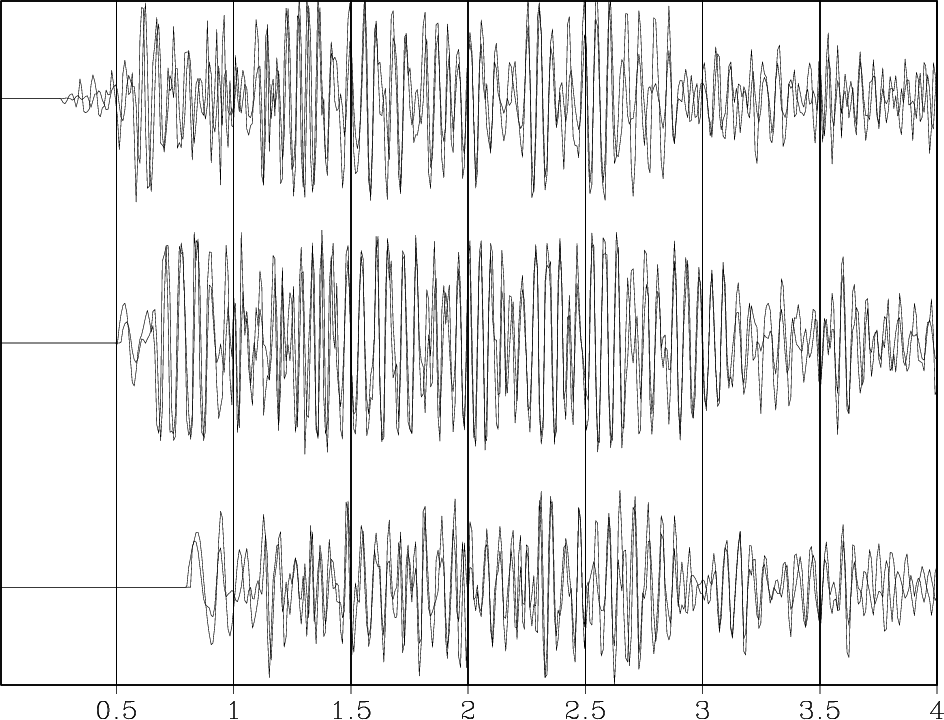
The following example uses transp=y poly=y yreverse=y pclip=100 unit2=km unit1=s label1=Time label2=Offset:

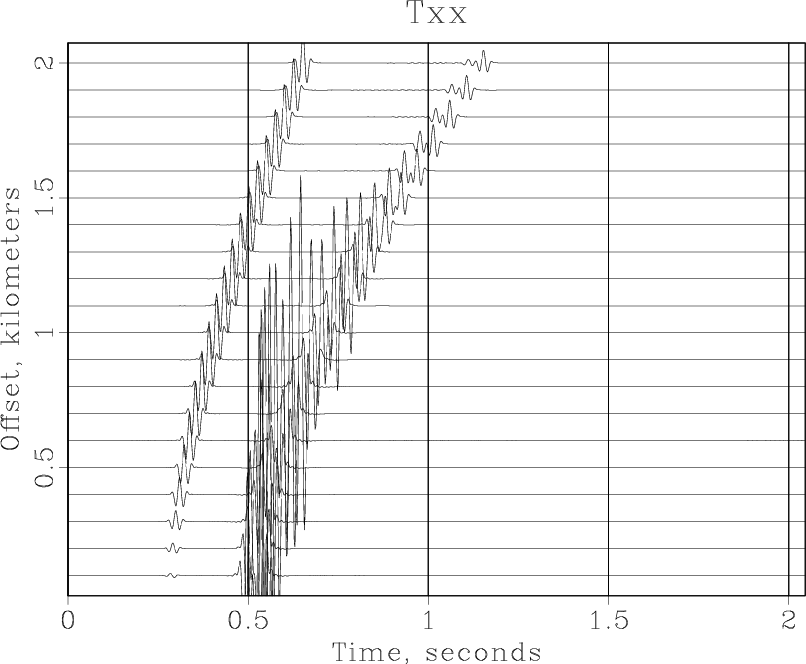
Use seemean=y to display lines corresponding to the mean value, use zplot= to control relative separation between different traces (the default is 0.75). The following example from bei/sg/toldi uses zplot=0.4:
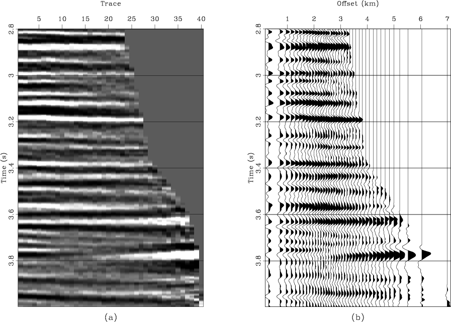
Finally, sfwiggle makes it possible to plot irregularly sampled data by providing trace coordinates in xpos= file and (optionally) coordinate range with xmin= and xmax=. The following example from jsg/avo/avo2 shows a seismic gather displayed with (a) sfgrey in trace-number coordinates and (b) sfwiggle in offset coordinates.
10 previous programs of the month:
Elastic wave equations on GPU
June 11, 2013 Documentation No comments
A new paper is added to the collection of reproducible documents:
Solving 3D anisotropic elastic wave equations on parallel GPU devices
This is the first contribution from the University of Western Australia.