|
|
|
|
Probabilistic moveout analysis by time warping |
Next: SEAM Phase II unconventional Up: Examples Previous: 2D Mobil Viking Graben
|
|
|
|
Probabilistic moveout analysis by time warping |
 ,
,  ,
,  , and
, and  are non-zero and can represent the case of an orthorhombic subsurface with azimuthally rotated principal axes with respect to the local Cartesian coordinates. The inputs of the time-warping workflow for this experiment have previously been used in our explanation on the method and are shown in Figure 1. We purposefully specify three CMP events at
  , 1.5, and 2
  , which correspond to the maximum offset-to-depth ratios of approximately 2.326, 1.789, and 1.5 in the
  direction and of 2.474, 1.876, and 1.5625 in the
  direction reflecting our choice of
  and
and  , respectively. According to the general rule of thumb of offset-to-depth ratio
  1 for nonhyperbolic moveout analysis (Tsvankin, 2012; Thomsen, 2014; Alkhalifah, 1997), we anticipate that our inverted posterior probability distributions for from the topmost event should demonstrate the best performance. We also add Gaussian noise with
  = 2.5 (top event), 2.75 (middle event), and 3.0 (bottom event) to the input traveltime data from automatically picked moveout curves. Because we are dealing with a more challenging 3D gather, we anticipate that the automatically picked moveout curve will no longer be error-free and therefore, the final estimates of would reflect total data uncertainty from both the artificially added noise and the automatic picking process.
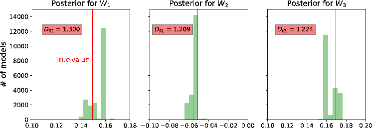
In this example, we specify the minimum and maximum values for the prior distributions as shown in Table 2. Here, we use the computational experiments with 3D GMA from Sripanich et al. (2017), as well as equation 13, to provide a rough estimate for the magnitude of each parameter and guide our choices of their min and max values, while keeping a relatively large range. The model parameters are recorded every 500 iterations until reaching a total of 20,000 models. The cutoff offsets for the first inversion in our workflow are at 1, 1.25, and 2 km for the top, middle, and bottom events, respectively. The estimated posterior probability distributions of the three events from our proposed workflow are shown in the form of histograms in Figures 11 – 16. It is apparent from Figure 11 that the are estimated well with relatively high  values.
| Parameters | |
 |
|
 |
 |
 |
 |
 |
 |
 |
 |
 |
 |
 |
 |
 |
|
|
| Min | 0.1 | -0.15 | 0.12 | -0.09 | -0.045 | -0.05 | -0.035 | -0.09 | 0.25 | 0.01 | 0.25 | 0.0015 | 0.001 | 0.0045 | 0.001 | 0.0015 | 0.0 | |
| Max | 0.3 | 0. | 0.32 | -0.001 | -0.02 | -0.03 | -0.015 | -0.001 | 0.8 | 0.1 | 0.75 | 0.005 | 0.0045 | 0.007 | 0.0035 | 0.0045 | 5 |
|
|---|
|
Whist0,Whist1,Whist2
Figure 11. A comparison of estimated posterior probability distributions for in the form of histograms for events at (a) 1 , (b) 1.5 , and (c) 2 of the 3D inverse moveout model. The solid vertical lines denote the true values.
|
|
|
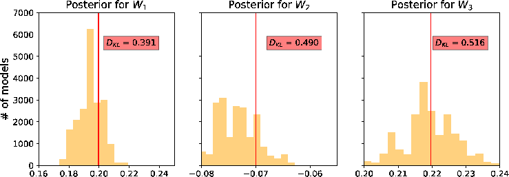
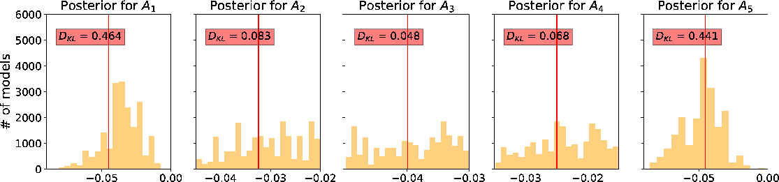
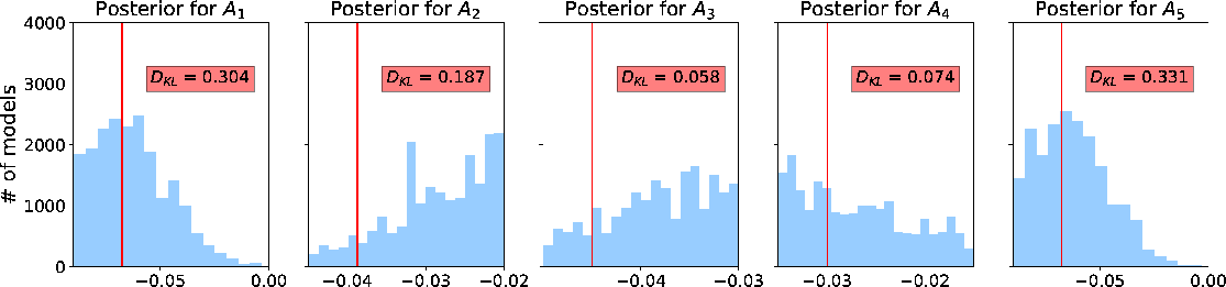
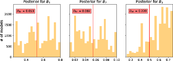
We proceed with the second inversion run with all available data and the resulting from the first run. The inverted from this experiment require more detailed analyses. First, we emphasize that the posterior distributions of appear more diffuse and multi-modal (Figure 12). This observation suggests that there are many equivalently good values of that can lead to an accurate prediction of the moveout traveltime, which indicates the inherent non-uniqueness of moveout inversion problem based on traveltime data alone. Moreover, it is not obvious that having a larger offset-to-depth ratio (Figure 12a associated with the topmost event) helps to mitigate this non-uniqueness of possible solutions.
|
|---|
|
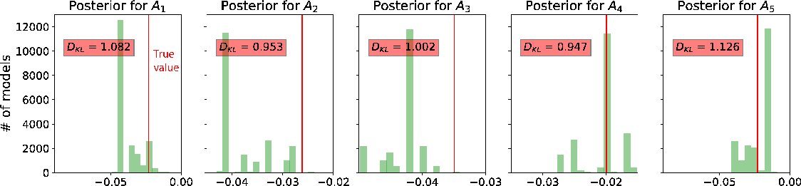
Ahist0,Ahist1,Ahist2
Figure 12. A comparison of estimated posterior probability distributions for in the form of histograms for events at (a) 1 , (b) 1.5 , and (c) 2 of the 3D inverse moveout model. Note that they are more diffuse than the inverted in Figure 11. The solid vertical lines denote the true values.
|
|
|
A closer look at Figures 11a, reveals that the peak of the posterior distribution of are slightly higher than the true value, whereas that of is slightly lower. This becomes less obvious in Figures 11b and 11c, which correspond to smaller offset-to-depth ratios. One explanation of this behavior can be given by considering Figures 11a and 12a together. In Figures 12a, the maximum likelihood values of the posterior also slightly deviate from the true values. Therefore, similar to the previous to 2D case, there appears to be a trade-off between inverted and on top of the non-uniqueness of possible solutions, which seems to be noticeable with data from larger offset-to-depth ratio. This observation is supported by the 2D marginal posterior distributions of and shown in Figure 13, where we can observe clear correlations between the  pair and the
  pair. A decrease in estimated () correlates with an increase in estimated (). A lesser degree of correlations can also be seen from
 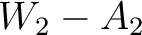 and
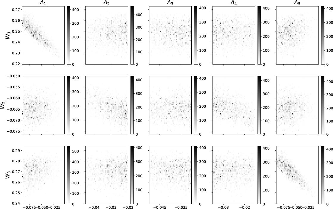
and 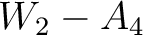 pairs, where a decrease in correlated with an increase in and . Correlations among other pairs of and are not observed from this experiment. Note that we display the 2D marginal posterior distributions from the bottom event at 2 in Figure 13. This is done to facilitate the visualization of possible correlations because the associated posterior distributions are more diffuse. However, our observation remains valid and applicable to other events because this trade-off behavior is a consequence of our inversion configuration with the 3D GMA.
|
|---|
|
thistmarginalW-A
Figure 13. 2D marginal posterior distributions of and from the 3D inverse moveout example for the event at 2 that suggest correlations and trade-offs among inverted parameters. The rows denote and the columns denote . Prominent correlations between the pair and pair can be observed.
|
|
|
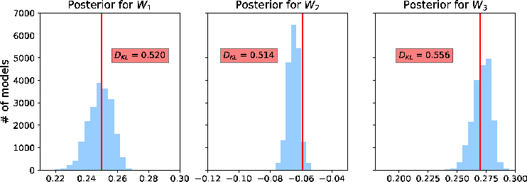
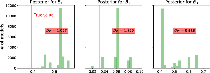
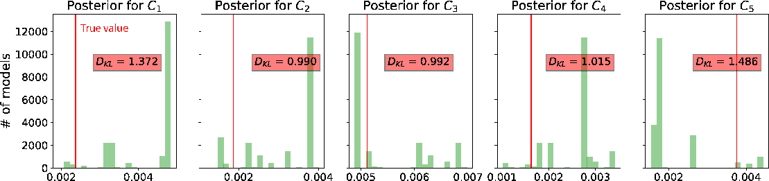
Analogous to the estimated , the resulting distributions of (Figure 14) and (Figure 15) are also fairly diffuse and multi-modal. Therefore, similar conclusions can be drawn regarding the non-uniqueness of possible solutions. However, similar to the 2D case, we emphasize that both parameters, whose values depend on the choice of finite-offset rays, are designed to be dynamic in the 3D GMA and this behavior is to be expected. Figure 16 shows the resulting posterior distributions of for the three events. We can observe that the peak estimates of are slightly higher than the level of added Gaussian noise agreeing with our expectation that the automatically picked moveout curve for this 3D gather contains a small degree of uncertainty, which can be captured and quantified in our workflow.
|
|---|
|
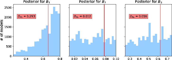
Bhist0,Bhist1,Bhist2
Figure 14. A comparison of estimated posterior probability distributions for in the form of histograms for events at (a) 1 , (b) 1.5 , and (c) 2 of the 3D inverse moveout model. Note that they are moderately diffuse and sometimes multi-modal similar to Figure 12. The solid vertical lines denote the true values.
|
|
|
|
|---|
|
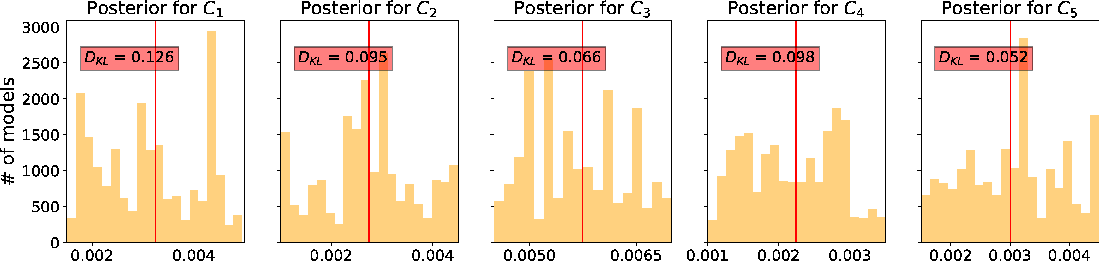
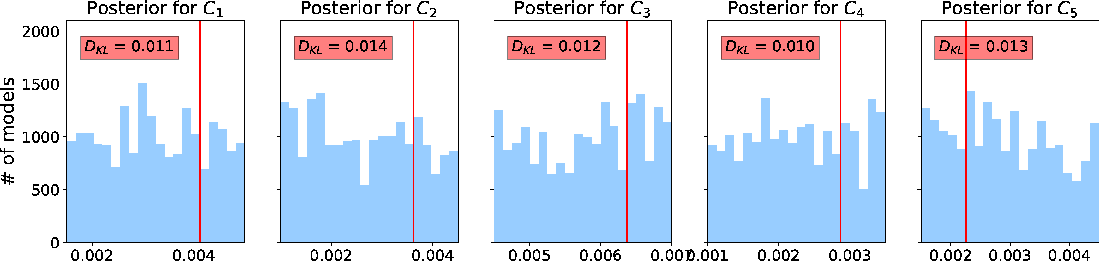
Chist0,Chist1,Chist2
Figure 15. A comparison of estimated posterior probability distributions for in the form of histograms for events at (a) 1 , (b) 1.5 , and (c) 2 of the 3D inverse moveout model. Note that they are moderately diffuse and sometimes multi-modal similar to Figure 12. The solid vertical lines denote the true values.
|
|
|
|
|---|
|
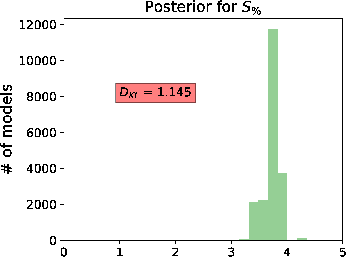
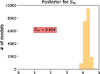
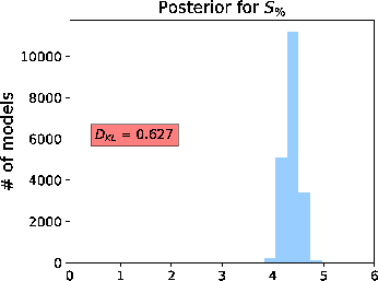
Shist0,Shist1,Shist2
Figure 16. A comparison of estimated posterior probability distributions for in the form of histograms for events at (a) 1 , (b) 1.5 , and (c) 2 of the 3D inverse moveout model reflecting the total uncertainty from both the automatically picked 3D moveout curve and the artificially added Gaussian noise. The peaks in the distributions are slightly higher than the levels of added Gaussian noise for the three events at = 2.5, 2.75, and 3 suggesting the small degree of uncertainty from the automatic picking process in a more challenging case of 3D gather.
|
|
|
We emphasize that the above analysis is permissible due to the use of a Bayesian framework for the inversion that gives posterior probability distribution as a result. Together with our analysis from the previous 2D inverse moveout example, our results suggest a limitation of using moveout traveltime inversion to estimate quartic coefficients, which becomes more difficult in 3D with a higher number of wanted parameters associated with a more complex subsurface model (e.g., orthorhombic media).
|
|
|
|
Probabilistic moveout analysis by time warping |