Time-warping workflow

Steps to implement the entire time-warping workflow can be summarized (Figures 1 and 2) as follows (Burnett and Fomel, 2009):

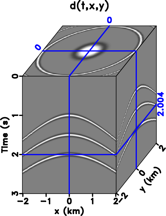
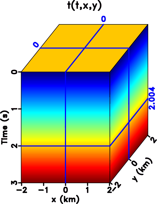
1. The inputs of the workflow include a CMP gather $d(t,x,y)$ and a time attribute volume as shown in Figures 1a and 1b. The latter is generated simply by having a similarly-sized volume as the CMP gather with each element storing the corresponding value of traveltime along the axis. After warping, this volume will store the reflection traveltimes from different CMP events.

2. Apply slope estimation on the CMP gather (Figure 1a) using tools such as plane-wave destruction filter (Fomel, 2002). The resulting slopes indicate the local structures and are used to automatically trace the CMP events in the predictive painting method (Fomel, 2010).

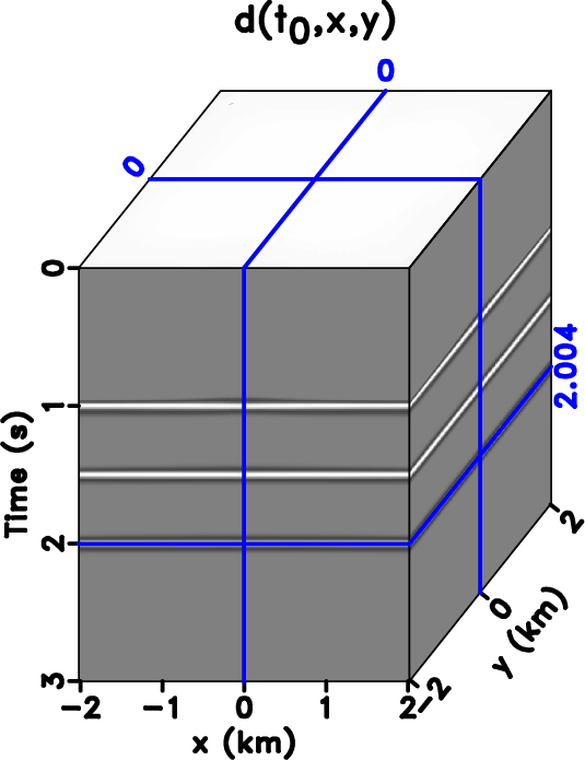
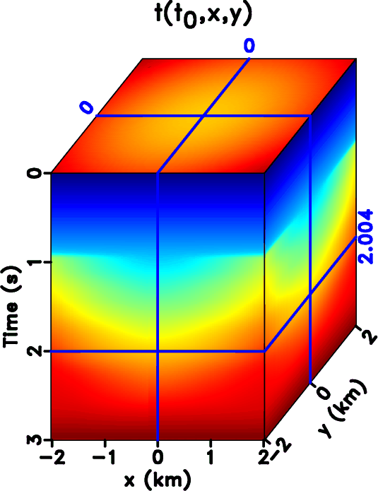
3. The picked events are then numerically warped until flattened by inverse interpolation. The warping process can be viewed as applying a nonstationary shifting filter. An application of this filter to $d(t,x,y)$ produces $d(t_0,x,y)$ in Figure 2a. Applying the same filter to the time attribute volume in Figure 1b, we obtain $t(t_0,x,y)$ in Figure 2b. Here, we restrict our application of warping to only the parts with CMP events between time 1 and 2 $s$.

4. In the considered time range (1–2 $s$), we can compute the traveltime shift volume by the element-wise subtraction of $t^2(t_0,x,y)-t_0^2$.

5. The resulting traveltime shifts will be used in the left-hand side of equation 2 for the moveout parameter inversion.

cmpcube,timecube
Figure 1. Original volumes of (a) CMP data $d(t,x,y)$ and (b) time attribute .

flat3cube,warpedtimecube
Figure 2. Warped volumes of (a) flattened CMP $d(t_0,x,y)$ and (b) time $t(t_0,x,y)$. We only apply warping to the time range of 1–2 $s$ because CMP events are present only in this $t_0$ range.

The above five steps are carried out in the same way, regardless of the choice of moveout approximation. These steps could also be applied to migrated common-image-point gathers, or many other gather or domain types. In this study, we focus on its application to the problem of moveout inversion, which is dependent upon the choice of moveout approximation $F$ and the inversion method. Different moveout approximations represent different shapes of reflection traveltime surfaces and involve a different number of moveout parameters to be fitted. An appropriate inversion method must also be chosen in accordance with the choice of moveout approximation. Whereas Burnett and Fomel (2009) solved for the three parameters of NMO ellipse moveout model using least-squares inversion, here we use a Monte Carlo inversion to infer the many parameters of the more comprehensive 3D GMA model.