SEAM Phase II unconventional reservoir model

For a more complex example, we consider a CMP gather from the 3D SEAM II unconventional reservoir model shown in Figure 17 (Oristaglio, 2015). This model has a largely flat structure suitable for moveout analysis and includes unaligned orthorhombic sublayers that require 3D multi-azimuth processing. 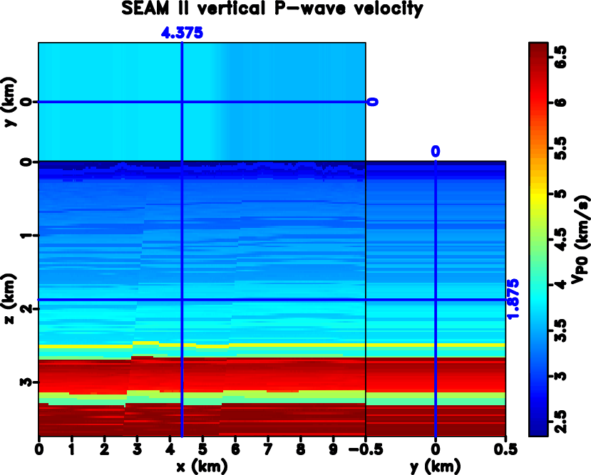We choose one CMP gather located at $x=4.735$ km and $y=2.881$ km, eliminate multiples, and bin to 39 $\times$ 39 offset samples from -3.8 km to 3.8 km in both $x$ and $y$ directions. We note that the maximum depth of this model is 3.75 km, therefore the offset-to-depth ratio of intermediate layers are moderately larger than unity.

vpseam3d
Figure 17. Vertical P-wave velocity of SEAM II unconventional reservoir model.

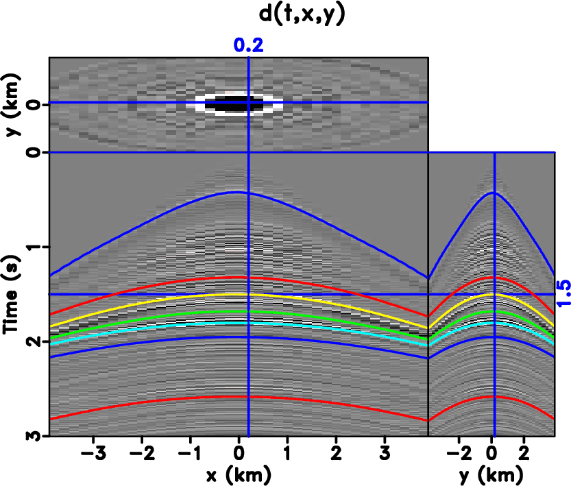
Figure 18 shows the considered CMP gather overlain by automatically traced events for non-physical flattening. We specifically focus on two events at $t_0$=1.315 s and 1.815 s. The parameter ranges for prior distributions are given in Table 3, where we use the same notion as in the previous 3D inverse moveout case to choose the min and max values. We also assume that $B_i$ and $C_i$ are largely unknown and specify relative large ranges for their values. The model parameters are recorded every 500 iterations until reaching a total of 10,000 models. The cutoff offsets for the first inversion are at 0.89 km and 1.5 km for the two events, respectively. In this example, we choose to use 1D average values of moveout parameters to benchmark our results. These values are computed by taking the true model parameters at the considered CMP location and use them to compute effective moveout parameters appropriate for a stack of horizontally layered unaligned orthorhombic media (Sripanich and Fomel, 2016; Koren and Ravve, 2017). They are exact in the case of truly 1D media but represent good approximate values of moveout parameters in this case of mildly laterally heterogeneous SEAM II model. We note also that in this example, the contribution from the quartic terms ($A_i$) as shown in their 1D average values are relatively small in comparison with that from the second-order terms ($W_i$). Therefore, this condition is expected to further hamper the parameter estimation process in addition to the inherent non-uniqueness of possible solutions.

pickongather0
Figure 18. The CMP gather of SEAM II model at $x$=4.375 km and $y$=2.881 km overlain by automatically picked events for non-physical flattening.

!

Parameters	$W_1$	$W_2$	$W_3$	$A_1$	$A_2$	$A_3$	$A_4$	$A_5$	$B_1$	$B_2$	$B_3$	$C_1$	$C_2$	$C_3$	$C_4$	$C_5$	$S_{\%}$
Min	0.05	-0.05	0.05	-0.01	0.0	-0.005	0.0	-0.01	0.0	0.0	0.0	0.0	0.0	0.0	0.0	0.0	0.0
Max	0.15	0.05	0.15	0.0	0.001	-0.001	0.001	0.0	0.5	0.1	0.5	0.005	0.005	0.005	0.005	0.005	5.0

Table 3. Minimum and maximum values of moveout parameters that define the uniform prior distributions for our Monte Carlo inversion for SEAM II example.

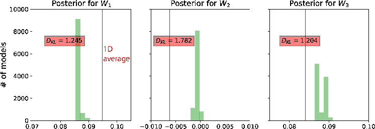
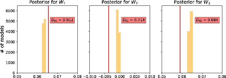
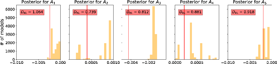
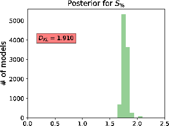
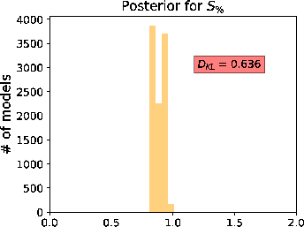
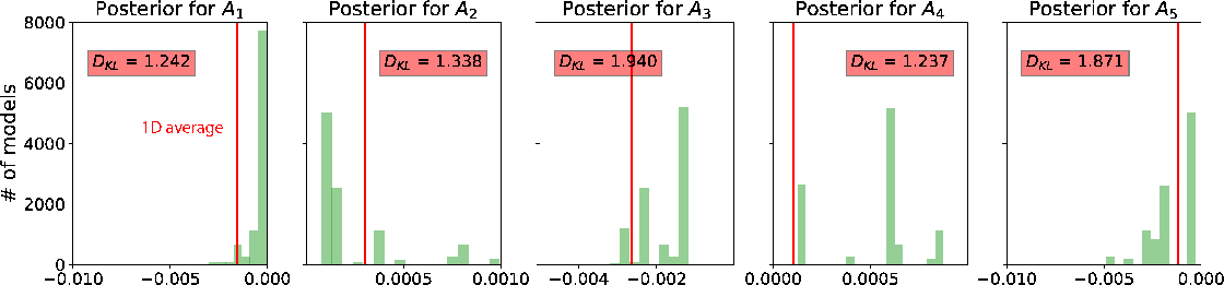
Example posterior histograms for events at $t_0=1.315$ $s$ and 1.815 $s$ are shown in Figures 19–21. It follows from the results that in this example of SEAM II, the proposed approach can capture $W_1$ and $W_3$ with clearly defined maximum likelihood values close to the 1D average values and a high value of $D_{KL}$. However, results on $W_{2}$ parameter that define the orientation of the NMO ellipse suggest that its value is centered around zero different from the 1D average value. The estimated posterior distributions of $A_i$ related to subsurface anisotropy exhibits the same characteristics as before — diffuse and multi-modal, although several maximum likelihood values and the 1D average values fall within the same ballpark. Agreeing with our previous analysis on 3D synthetic example, these results suggest that it is possible to estimate the quartic moveout coefficients from a 3D gather associated with complex anisotropic media, although there is a limitation on the inherent non-uniqueness of solutions due to more diffuse and and multi-modal posterior distributions in comparison with $W_i$, which are generally well-constrained.

Whist0seam,Whist1seam
Figure 19. A comparison of estimated posterior probability distributions for $W_i$ in the form of histograms for events at (a) 1.315 $s$ and (b) 1.815 $s$ of the SEAM II model. The solid vertical lines denote the 1D average values.

Ahist0seam,Ahist1seam
Figure 20. A comparison of estimated posterior probability distributions for $A_i$ in the form of histograms for events at (a) 1.315 $s$ and (b) 1.815 of the SEAM II model. They are not as well-constrained as the inverted $W_1$ and $W_3$, which indicate large uncertainties. The solid vertical lines denote the 1D average values.

Shist0seam,Shist1seam
Figure 21. A comparison of estimated posterior probability distributions for $S_{\%}$ in the form of histograms for events at (a) 1.315 $s$ and (b) 1.815 of the SEAM II model.