2D Mobil Viking Graben data set

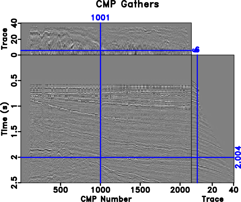
Next, we consider an example with real 2D dataset from the Viking Graben (Figure 7) from Keys and Foster (1998). In this example, we utilize the flexibility of the proposed time-warping workflow that can be implemented at any selected locations related to different reflectors to help assessing velocity estimated from conventional semblance-based technique. We can achieve this selection by choosing an appropriate $t_0$ (a slice of the $t(t_0,x,y)$ cube) that corresponds to the desired reflector and implement a Monte Carlo inversion only at such location.

cmpsvk
Figure 7. The Mobil Viking Graben dataset.

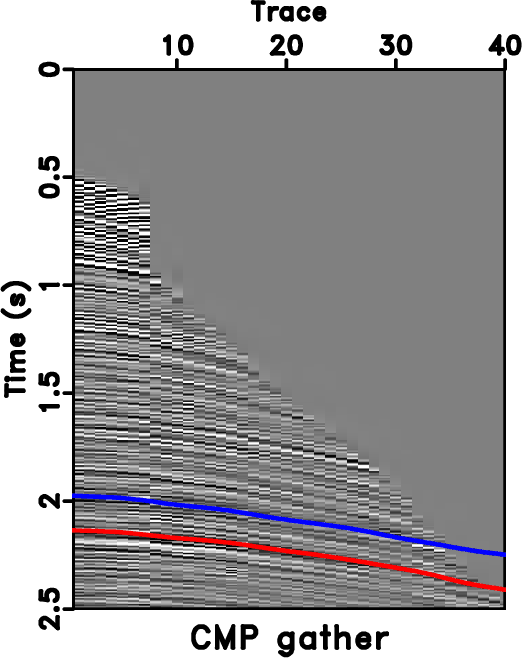
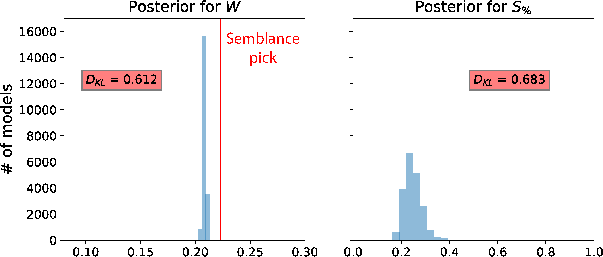
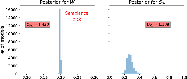
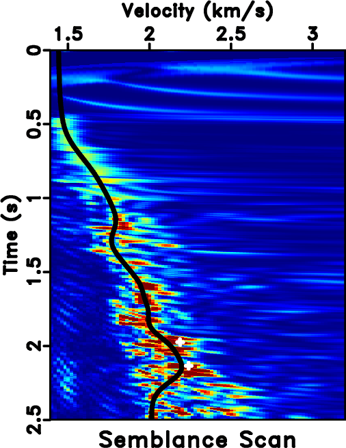
Figure 8 shows the CMP gather number 1000 of the Viking Graben data overlain by two picked moveout curves associated with prominent reflectors to be considered in our inversion. Due to the availability of only small-offset data, we are obliged to restrict our inversion to $W$ and $S_{\%}$. Their ranges for the input uniform prior distribution are 0.08–0.5 for $W$ and 0–10 for $S_{\%}$. The cutoff offsets used for the two events are at 1.8 (blue) and 2.2 km (red) approximately corresponding to trace number 27 and 35, respectively. A comparison of the semblance-based velocity and those from the proposed workflow is shown in Figure 9 with the solid black line denoting semblance-based velocity picks and white `+' signs denoting the maximum likelihood points from the proposed inversion workflow. The estimated posterior distributions of both events are shown in Figure 10. We can see that in this example the results from both approaches generally agree well with each other despite relying on different theoretical bases (signal coherency vs. traveltime-only inversion) to estimate $W$. This result gives further assurance to the estimated parameters. Nevertheless, we note that using the proposed workflow, we obtain posterior distributions that contain additional statistical information for more assessment and quality control of both the estimated moveout parameters (only $W$ in this case) and the input data uncertainty ($S_{\%}$).

pickvk
Figure 8. CMP number 1000 from the Mobil Viking Graben dataset overlaid by picked moveout curve used in the time-warping workflow. The cutoff offsets at 1.8 (for blue) and 2.2 (for red) km are approximately at trace number 27 and 35.

vscanvk
Figure 9. Semblance scan and automatically picked velocity (black line) associated with CMP number 1000 from the Mobil Viking Graben dataset. The white `+' signs are the peaks of estimated posterior distribution of $W$ from the proposed inversion workflow.

thistviking-1,thistviking-2
Figure 10. Estimated posterior probability distributions in the form of histograms for the (a) blue and (b) red events (Figure 8) associated with CMP number 1000 from the Mobil Viking Graben dataset. The solid lines denote picked values from semblance-based analysis.