|
|
|
|
Probabilistic moveout analysis by time warping |
Next: 2D Mobil Viking Graben Up: Examples Previous: Examples
|
|
|
|
Probabilistic moveout analysis by time warping |
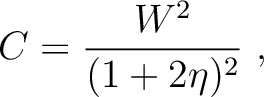
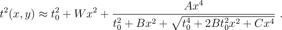
We first consider a simple 2D example where the input CMP gather is generated from the inverse moveout process based on the 2D version (Fomel and Stovas, 2010) of equation 4 (2D GMA) given by
This case can be associated with a horizontal reflector beneath a homogeneous layer of transversely isotropic medium with vertical symmetry axis (VTI). Relying on the pseudoacoustic approximation and the choice of zero-offset and horizontal rays to fit moveout parameters, Fomel and Stovas (2010) show that for a homogeneous VTI medium, it is possible to specify ,
,  , and
, and  in terms of
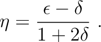
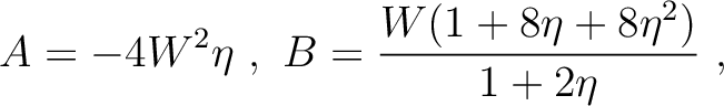
  (Alkhalifah and Tsvankin, 1995) — a commonly used parameter to characterize the nonhyperbolicity of moveout traveltimes. This process leads to
where
(Alkhalifah and Tsvankin, 1995) — a commonly used parameter to characterize the nonhyperbolicity of moveout traveltimes. This process leads to
where
 |
(14) |
 and
and  are Thomsen's parameters that characterize the property of the overlying VTI medium.
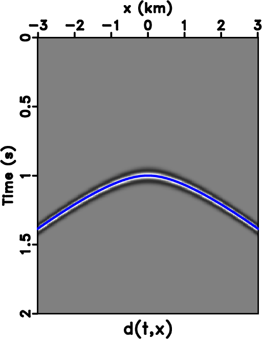
In this example, we consider a CMP event generated by the inverse moveout process (Figure 3) based on the 2D GMA (equation 12) with , , and specified as in equation 13. We use the VTI parameters of Dry Green River shale (Thomsen, 1986) given by
 km/s,
km/s,
 km/s,
km/s,
 , and
, and
 . These numbers can be translated to
 km/s and
 , which by equation 13, correspond to
  ,
, 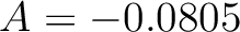 ,
, 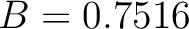 , and
, and 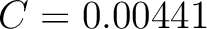 .
.
|
|---|
|
pick2d
Figure 3. The CMP gather 2D Dry Green River shale VTI model overlain by an automatically picked event (blue) for non-physical flattening. |
|
|
Using this configuration, we first test our algorithm and its capability to estimate both wanted model parameters and the hyperparameter  that governs the data uncertainty. We consider the setup for the first inversion run in our workflow, where we restrict our data range to small offsets. The benefit of this test is two-fold:
 and , while seeing how the posterior distributions of changes with varying data uncertainty .
 (equation 8) with =0.1, 0.5, 2, 5, and 25 to the input
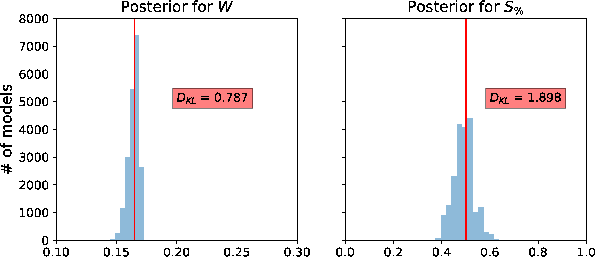
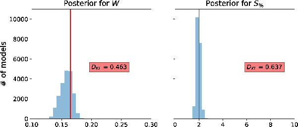
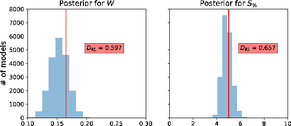
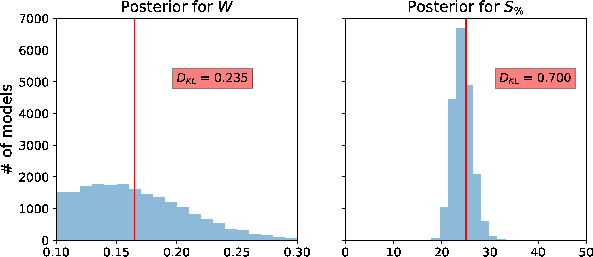
 for the inversion process. We record model parameters at every 100 iterations to increase the independence between recorded models and stop the iterations when the number of recorded model reaches 20,000. We specify the minimum and maximum values for the uniform prior distributions as shown in Table 1 except for the range of , which is set to 0–60 in this case. Here, we use the relationships between GMA parameters (, , and ) and (equation 13) to help guide our selection of the min and max values and we also specify relatively large ranges to reflect the reality of this situation in practice. The resulting posterior distributions for and from this experiment with the cutoff offset specified at 1.25 km are shown in Figure 4. We can observe that our algorithm performs well and manages to correctly estimate posterior distributions for both and centered around the true values. Moreover, at lower (small data uncertainty/noise), the estimated posterior distribution of has smaller variance and has its peak closer to the true value. On the other hand, the estimated posterior distribution of becomes wider (higher variance) with increasing as would be anticipated. Looking closer at Figure 4, we also see that at higher levels of , the peak of the posterior distribution of shifts towards lower value suggesting a trade-off between inverted parameters despite the use of only small-offset data. This observation is supported by the 2D marginal posterior distributions of and the other three parameters: , , and as shown in Figure 5 for the case of =2. We can observe a clear correlation between the
  pair. A decrease in estimated correlates with an increase in estimated suggesting a trade-off between the two parameters in our inversion setup. Correlations among the other pairs of
  and
and  are not observed in this experiment.
| Parameters | |
|
|
|
|
| Min | 0.1 | -0.1 | 0.5 | 0.0 | 0.0 |
| Max | 0.3 | 0.0 | 1.0 | 0.006 | 10 |
|
|---|
|
thistnoise2D-S01,thistnoise2D-S05,thistnoise2D-S2,thistnoise2D-S5,thistnoise2D-S25
Figure 4. A comparison of estimated posterior probability distributions for and of the Dry Green River shale example with cutoff offset at 1.25 km for different levels of added Gaussian noise with = (a) 0.1, (b) 0.5, (c) 2, (d) 5, and (e) 25. The solid vertical lines denote the true values.
|
|
|
|
|---|
|
thistmarginal2D
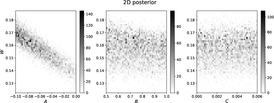
Figure 5. 2D marginal posterior distributions of and , , and . Prominent correlations between the pair can be observed suggesting trade-offs in estimating the two parameters.
|
|
|
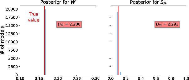
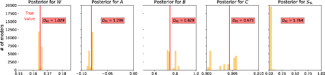
After successful testing, we use the same example and implement the proposed two-run inversion without any additional noise to the input data. In this case, we record the model at every 500 iterations and stop when the total number of recorded model reaches 20,000. Similar min and max values for the uniform prior distributions in Table 1 are used in this experiment. The resulting posterior distributions of all estimated parameters are shown in Figure 6. We can observe that the posterior distributions of and have their peaks close to the true values with high  suggesting that information on both parameters has been gained from the inversion and they appear to be recoverable relatively high fidelity. On the other hand, the distributions for and are more diffuse with no clear peak and lower . We emphasize that the results on and agree with the properties of the GMA, where both parameters are designed to be non-unique for dynamic traveltime fitting with high accuracy. Finally, the posterior distribution for has only one peak close to zero verifying our assumption that the picked traveltime curve in this example is approximately noise-free.
|
|---|
|
thist2D
Figure 6. Estimated posterior probability distributions in the form of histograms from the proposed two-run inversion for the Dry Green River shale example. The solid vertical lines denote the true values. The maximum likelihood points are located close to the true values suggesting that moveout parameters from 2D gathers are well recoverable from the proposed approach. |
|
|
|
|
|
|
Probabilistic moveout analysis by time warping |
 and
and