2D Field Data Example

To further test the proposed method, we use a common-midpoint gather from the North Sea dataset (Figure 15). Figure 16a shows the data in the seislet transform domain. We observe that significant coefficients are apparent in only a narrow area on the left, which indicates the excellent compression ability of the proposed RT formulation of the seislet transform. The field data reconstruction using only 1% of the most significant RT-seislet coefficients is shown in Figure 16b. The reconstructed image retains the most important seismic events in the original seismic data.

gath0
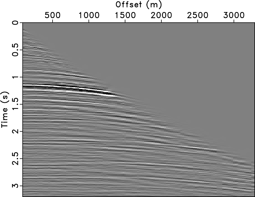
Figure 15. Common-midpoint gather.

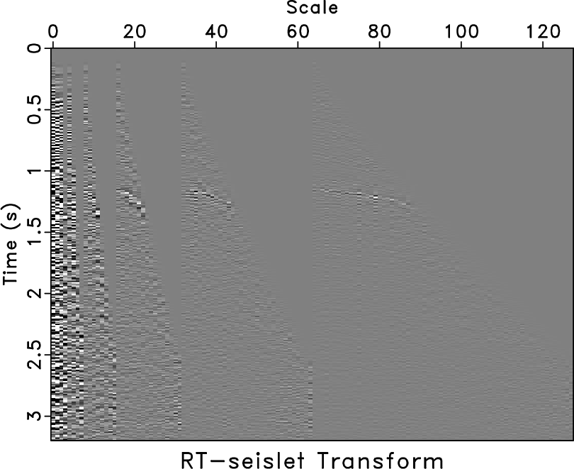
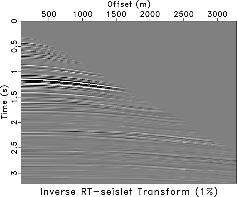
seis,seisrec1
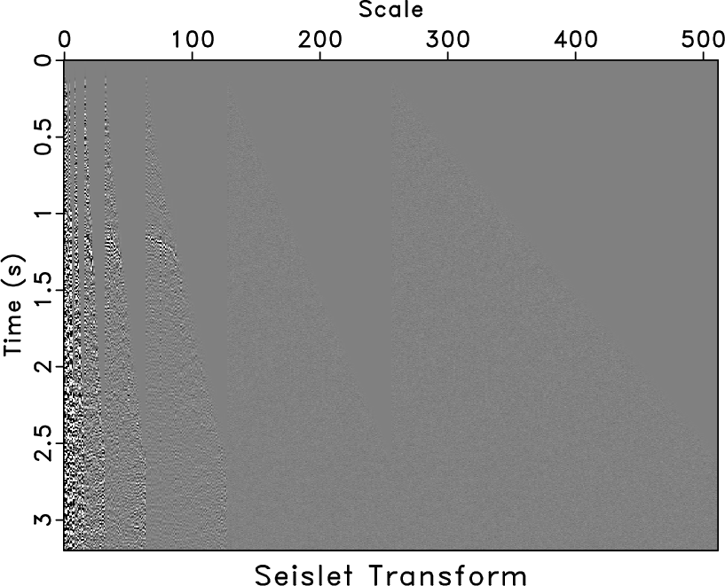
Figure 16. (a) The field data in the RT-seislet transform domain and (b) reconstruction using only 1% of significant coefficients by the inverse RT-seislet transform.

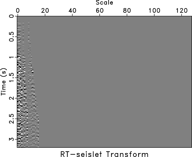
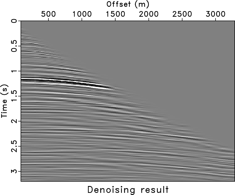
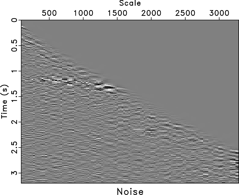
If we mute the RT-seislet coefficients at fine scales while keeping the significant coefficients at coarse scales (Figure 17b), the inverse RT-seislet transform enables effective denoising, removing incoherent noise from the gather. The result of denoising are shown in Figure 17c. Figure 17d shows the removed noise section using the proposed implementation of the seislet transform.

gath1,seisdeno,seis16,diff
Figure 17. (a) Original gather. (b) Denoised result by muting RT-seislet coefficients at fine scales (a) and (c) the removed noise section using the RT-seislet transform.

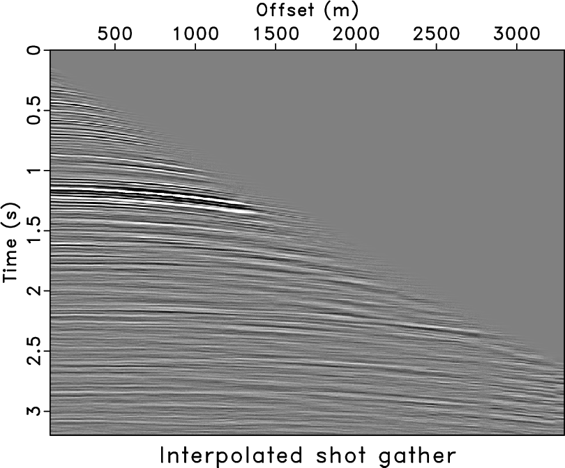
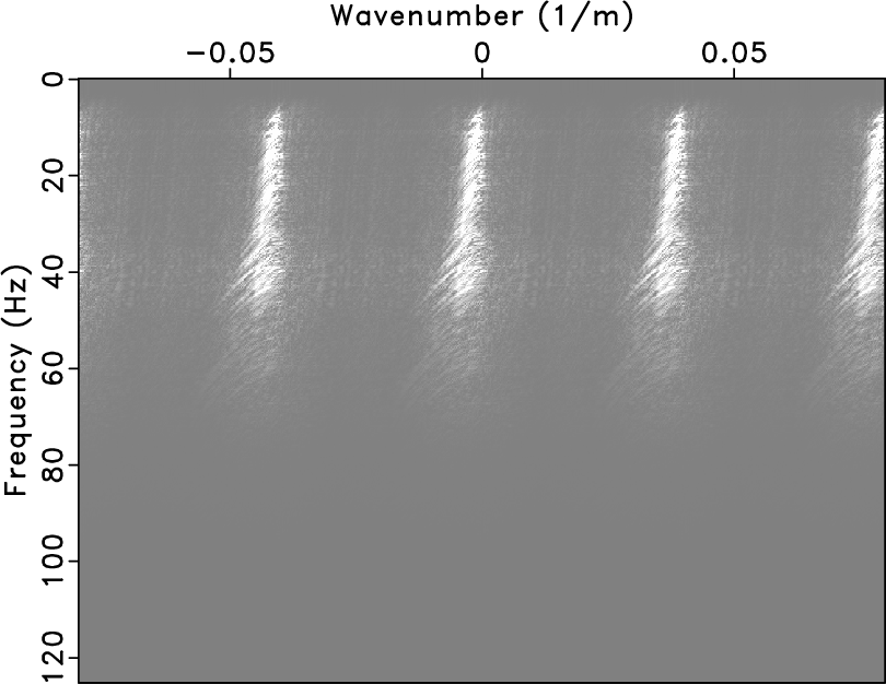
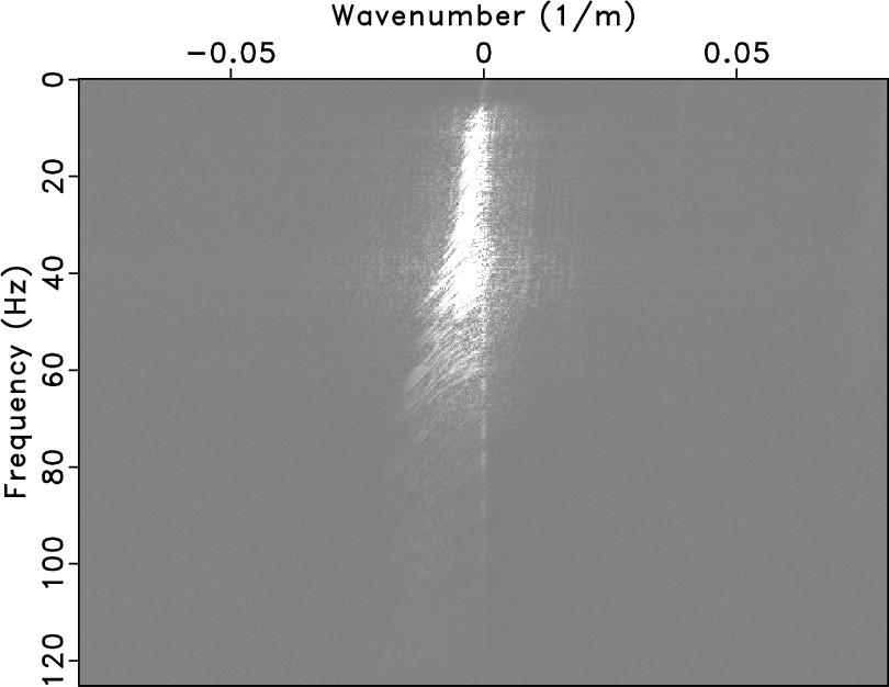
The RT-seislet is also able to perform interpolation. We add two more scales with small random noise to Figure 16a and interpolate the RT volume by a factor of four. Then the interpolated shot gather is obtained and the number of traces is increased by four. The extended data in the seislet transform domain is shown in Figure 18a. Figure 18b is the interpolated shot gather. Figure 19 shows the F-K spectrum of the zero-padded field data and the interpolated gather. The zero-padded shot gather is generated by manually padding zero traces between two traces. In this example, the seislet transform domain is extended with random noise because there is unpredictable noise in the real case.

seisrand2,gath4
Figure 18. (a) Extended seislet transform domain. (b) Interpolated shot gather by the inverse RT-seislet transform.

fft,fft2
Figure 19. F-K spectra of (a) zero-padded and (b) the interpolated field data.