|
|
|
|
Relative time seislet transform |
Next: Discussion Up: Geng et al.: RT-seislet Previous: 2D Field Data Example
|
|
|
|
Relative time seislet transform |
|
|---|
|
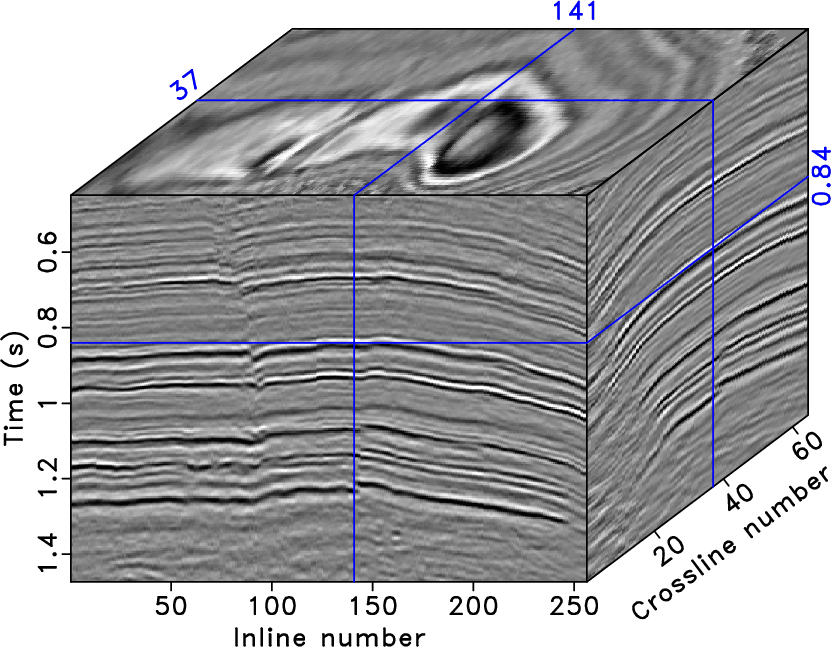
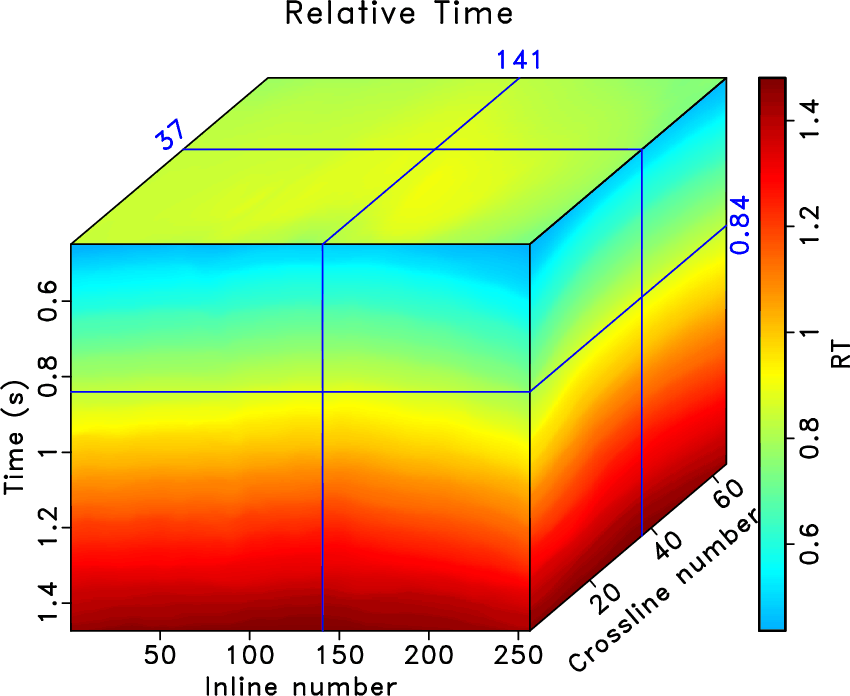
cuber,pick
Figure 20. (a) Teapot dome dataset. (b) RT volume estimated by the predictive painting. |
|
|
|
|---|
|
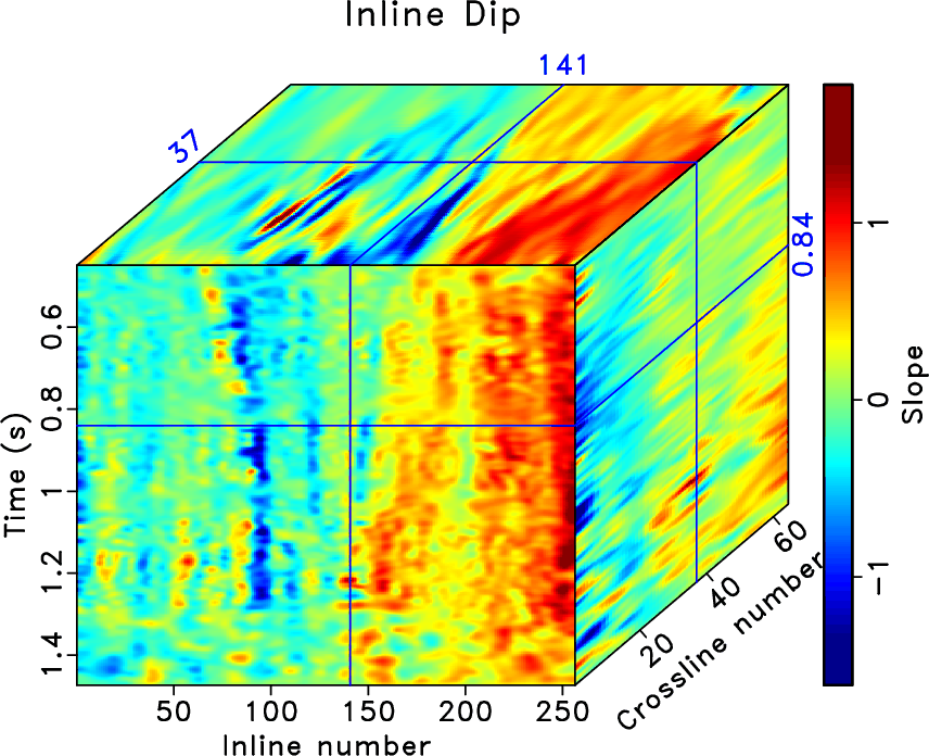
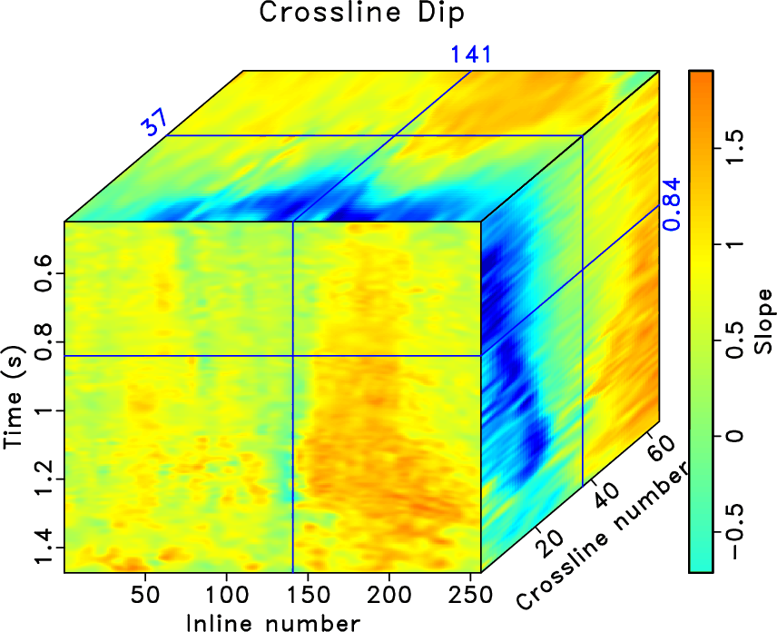
dip1,dip2
Figure 21. Inline (a) and Crossline (b) Dip. |
|
|
|
|---|
|
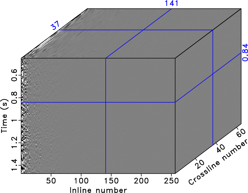
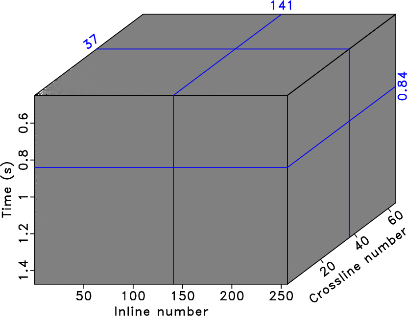
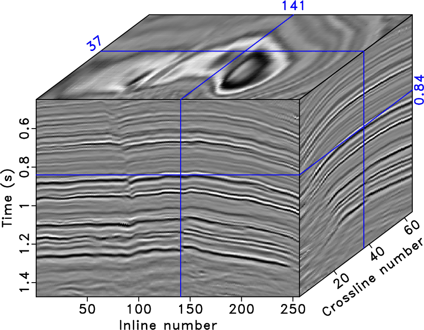
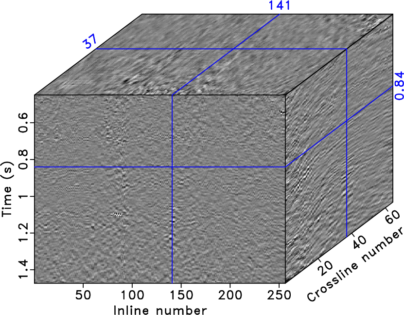
rtseis-inline,rtseis,teapot-rtseisrec5,teapot-diff
Figure 22. (a) The coefficients in 2D seislet domain along inline only. (b) The coefficients in 3D seislet domain. (c) Data reconstruction using only 5% of significant coefficients by the inverse RT-seislet transform. (d) Difference between (c) and the original seismic volume (Figure 20a). |
|
|
|
|
|
|
Relative time seislet transform |