|
|
|
|
Least-squares non-stationary triangle smoothing |
Next: Matching and merging low-resolution Up: Applications Previous: Non-stationary local signal and
|
|
|
|
Least-squares non-stationary triangle smoothing |
 is the wavefield,
  and
and  are time and space, and
  is the local slope. The general solution of equation 20 in the frequency domain is expressed as
This solution indicates a two-term prediction-error filter in the F-X domain
where
is the local slope. The general solution of equation 20 in the frequency domain is expressed as
This solution indicates a two-term prediction-error filter in the F-X domain
where  and
and
 .
The PWD prediction error filter can be transformed into the Z-transform notation as
where
.
The PWD prediction error filter can be transformed into the Z-transform notation as
where
 is an all-pass filter that allows equation 20 to be transformed into the following non-linear inverse problem
where
is an all-pass filter that allows equation 20 to be transformed into the following non-linear inverse problem
where
 is a convolutional operator that is non-linear with respect to . This non-linear problem can be solved for via the following least-squares method
where
is a convolutional operator that is non-linear with respect to . This non-linear problem can be solved for via the following least-squares method
where
 is the Jacobian matrix with respect to and can be expressed as
 where
where
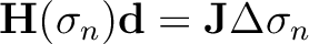
 is the derivative form of the PWD filter. A smooth and stable slope update can be obtained using the shaping regularization method
where
is the derivative form of the PWD filter. A smooth and stable slope update can be obtained using the shaping regularization method
where
 is the slope update at the
  th iteration and
 is a shaping operator. The solution according to the shaping regularization method is
where
is a shaping operator. The solution according to the shaping regularization method is
where
 is a non-stationary triangle smoothing operator.
Wang et al. (2021) propose designing a non-stationary smoothing constraint with the concept of signal reliability. The smoothing radius is meant to be small in areas where the signal dominates, and large in areas where the noise dominates. Wang et al. (2021) propose using the iterative radius estimation method of Greer and Fomel (2018), matching the local frequency of the low-pass filtered seismic data, and the seismic data smoothed via a non-stationary triangle smoothing operator. Wang et al. (2021) also introduce an additional re-scaling step to constrain the estimated radius between some chosen minimum and maximum values.
is a non-stationary triangle smoothing operator.
Wang et al. (2021) propose designing a non-stationary smoothing constraint with the concept of signal reliability. The smoothing radius is meant to be small in areas where the signal dominates, and large in areas where the noise dominates. Wang et al. (2021) propose using the iterative radius estimation method of Greer and Fomel (2018), matching the local frequency of the low-pass filtered seismic data, and the seismic data smoothed via a non-stationary triangle smoothing operator. Wang et al. (2021) also introduce an additional re-scaling step to constrain the estimated radius between some chosen minimum and maximum values.
We propose an alternative faster approach of obtaining the non-stationary smoothing constraint that estimates local slopes similar in accuracy to the slopes estimated using the approach of Wang et al. (2021). The proposed approach is summarized in the following three-steps: (1) estimating a noisy local slope using a small stationary radius, (2) applying a non-linear edge-preserving filter to the result of step 1 (e.g. fast explicit diffusion (Grewenig et al., 2010)), and (3) using the proposed Gauss-Newton method of estimating the non-stationary radius substituting the result of step 1 as
 and the result of step 2 as
 in equation 15. We justify this approach by noting that the result of step 1 contains detailed local slopes that are contaminated by high-frequency noise. The non-linear smoothing filter removes the high frequency noise while preserving strong edges. We note that the areas where the non-linear smoothing filter acts strongly are the areas of low signal reliability, while the areas where the filter acts weakly are the areas of high signal reliability. Thus, the non-stationary triangle filter defined by the estimated radius values is adaptive to signal reliability in the input dataset.
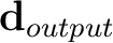
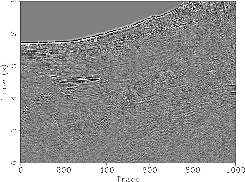
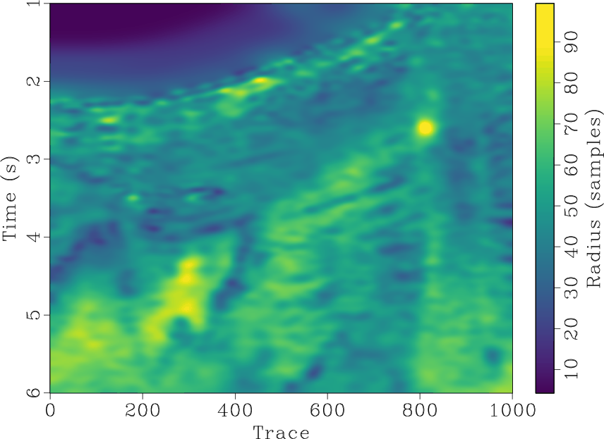
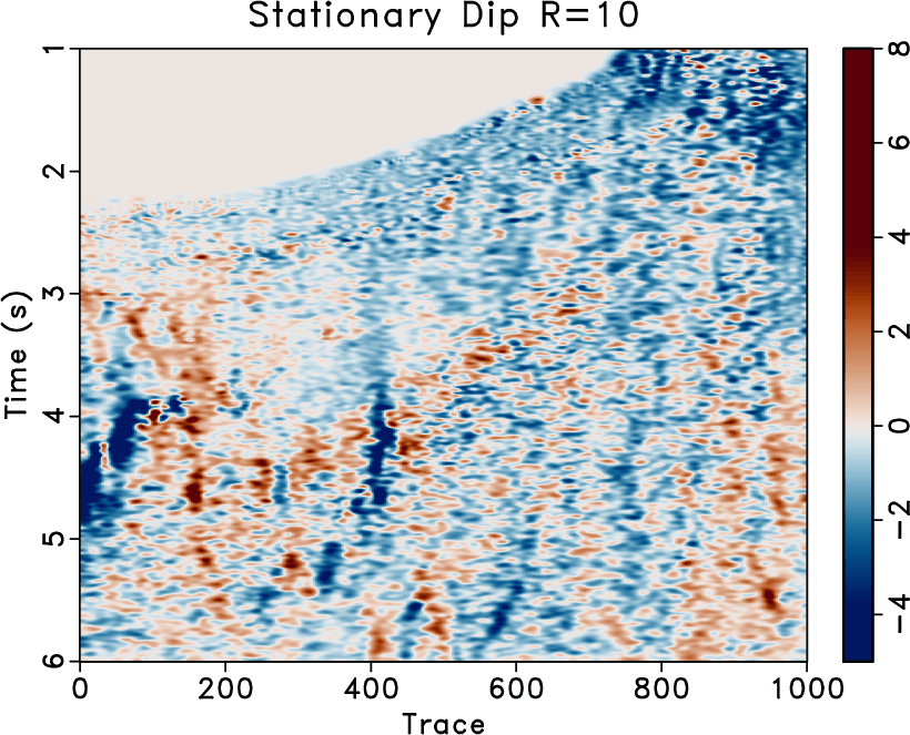
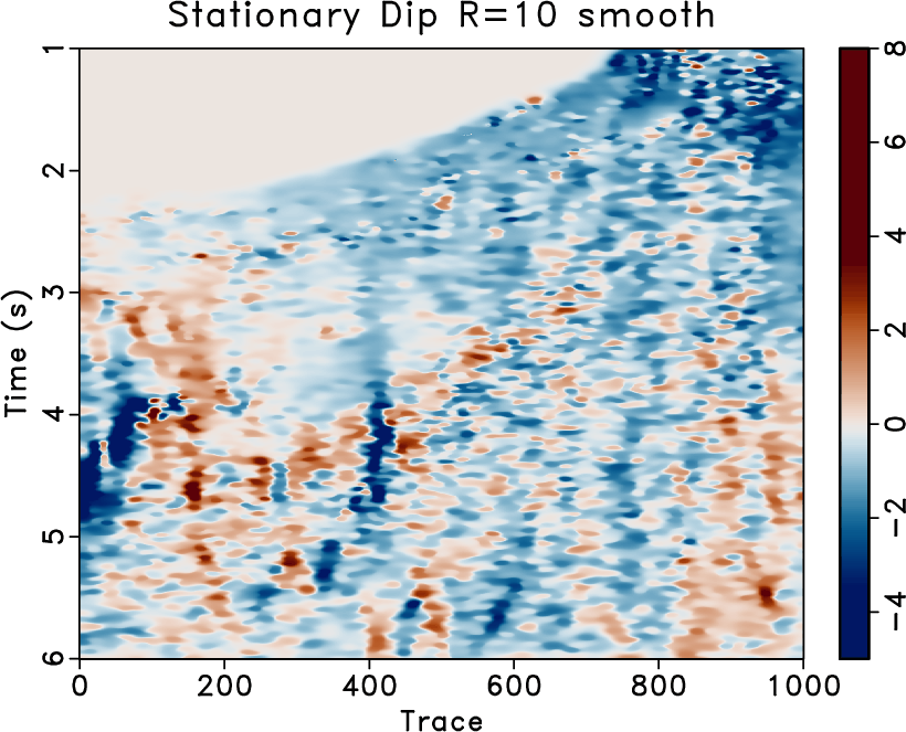
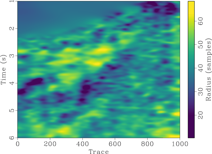
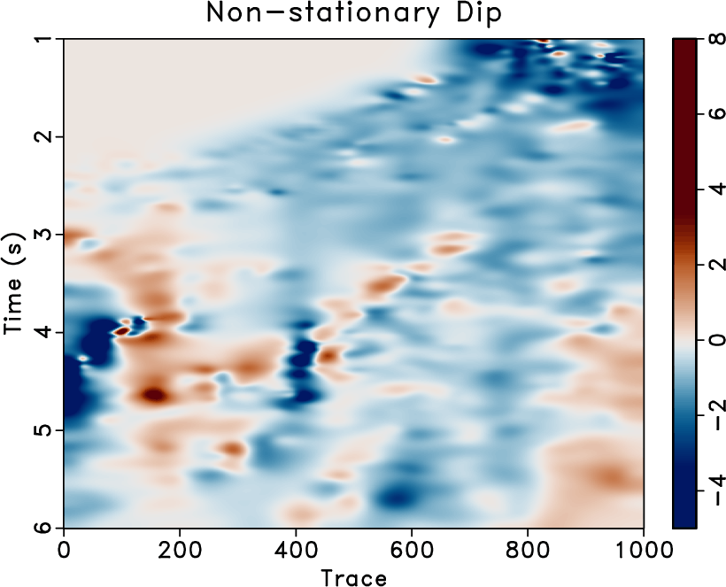
The proposed approach is evaluated on a 2-D field dataset displayed in Figure 9a. The estimated dip using a small stationary radius equal to 10 is displayed in Figure 10a, and the result of applying a fast explicit diffusion filter to the estimated stationary dip is displayed in Figure 10b. The non-stationary triangle smoothing radius obtained using 5 iterations of the proposed method matching the dip estimaeted using a small stationary radius and it's fast explicit diffusion filtered version is displayed in Figure 10c, and its corresponding estimated non-stationary dip is displayed in Figure 10d. For comparative analysis, the non-stationary radius obtained using the approach of Wang et al. (2021) and its corresponding estimated non-stationary dip is displayed in Figures 9b and 9c respectively.
|
|---|
|
g-high,g-rectdip1,g-dip3
Figure 9. Field data example 2. (a) Raw field data. (b) Estimated triangle smoothing radius using 5 iterations of the line-search approach proposed by Wang et al. (2021). (c) Estimated dip using non-stationary smoothing radius in (b). |
|
|
|
|---|
|
g-dip-test,g-dip-test-smooth,rect-dip1-new2,g-dip4
Figure 10. Field data example 2. (a) Estimated Dip using a small stationary radius equal to 12. (b) Estimated Dip using a small stationary radius equal to 12 smoothed by a bilateral filter. (c) Estimated triangle smoothing radius using 5 iterations of the proposed Gauss-Newton method matching (a) and (b). (d) Estimated Dip using non-stationary smoothing radius in (c). |
|
|
The estimated non-stationary slopes using the proposed approach and the approach of Wang et al. (2021) are similar from a visual standpoint. The main difference between the two approaches is in efficiency and robustness. In the iterative radius estimation approach of Wang et al. (2021), the local-frequency calculation step costs 6 s per iteration, adding up to a total cost of 30 s for 5 iteration. For the Gauss-Newton method, the cost per iteration is less than 0.1 s. The main cost associated with the proposed method is the initial computation of the estimated dip with a small stationary radius, and applying a non-linear smoothing filter to it, costing 6 s and 19 s respectively. Further, the proposed approach is more robust since we do not require any further analysis associated with re-scaling the estimated radius between a chosen minimum and maximum value.
|
|
|
|
Least-squares non-stationary triangle smoothing |
![$\displaystyle \Delta\sigma_{n}^{m}=\mathbf{S}[\Delta\sigma_{n}^{m-1}+\mathbf{J}^T(\mathbf{H}(\sigma_{n})\mathbf{d}-\mathbf{J}\Delta\sigma_{n}^{m-1})]$](img74.png)
![$\displaystyle \Delta\hat{\sigma}_{n}=\mathbf{T}[\lambda^2\mathbf{I}+\mathbf{T}^...
...athbf{I})\mathbf{T}]^{-1}\mathbf{T}^T\mathbf{J}^T\mathbf{H}(\sigma_n)\mathbf{d}$](img77.png)