|
|
|
|
Least-squares non-stationary triangle smoothing |
Next: Non-stationary local slope estimation Up: Applications Previous: Applications
|
|
|
|
Least-squares non-stationary triangle smoothing |
 and noise
 , the locally orthogonalized signal
 and locally orthogonalized noise
 can be expressed as
where
can be expressed as
where
 is the local orthogonalization weight (Chen and Fomel, 2015) and
  is the element-wise product.
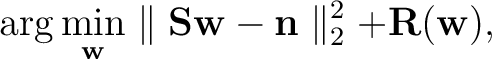
The local orthogonalization weight can be solved for via the following regularized least-squares problem (Chen and Fomel, 2021):
where
is the element-wise product.
The local orthogonalization weight can be solved for via the following regularized least-squares problem (Chen and Fomel, 2021):
where
 is the diagonal matrix of
 and
and
 is the regularization term.
Based on the shaping regularization method (Fomel, 2007b), the non-stationary local orthogonalization weight can be obtained as
where
is the regularization term.
Based on the shaping regularization method (Fomel, 2007b), the non-stationary local orthogonalization weight can be obtained as
where
 is a non-stationary triangle smoothing operator,
 is an identity matrix, and
 .
To obtain
, Chen and Fomel (2021) propose using the iterative radius estimation approach of Greer and Fomel (2018).
The approach of Greer and Fomel (2018) is based on an optimization problem solved by a line-search method that aims to minimize the difference in local frequency between the low-pass filtered seismic data and the seismic data smoothed via a non-stationary triangle smoothing operator.
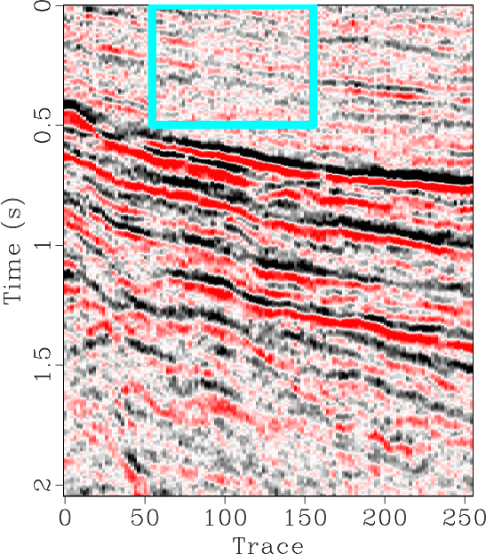
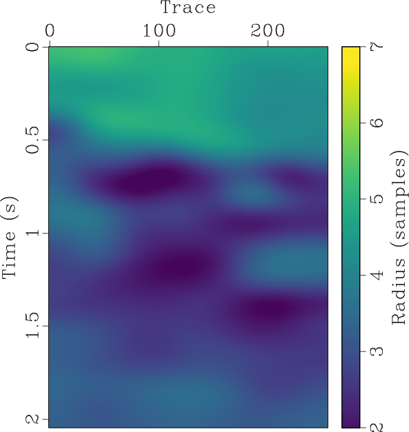
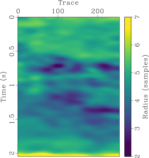
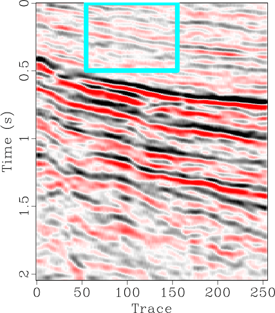
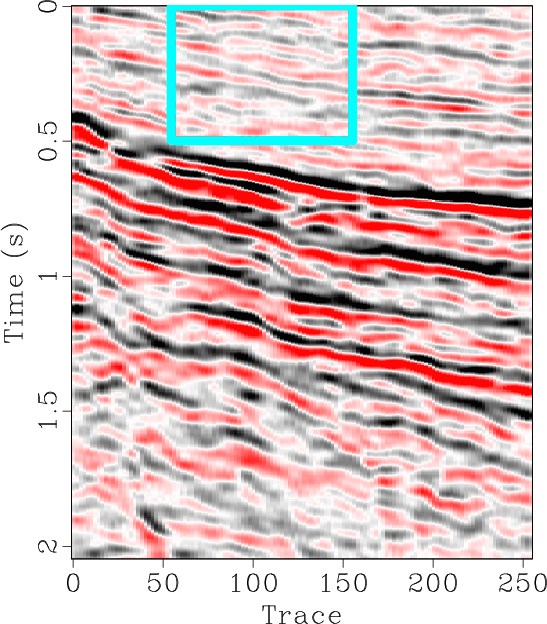
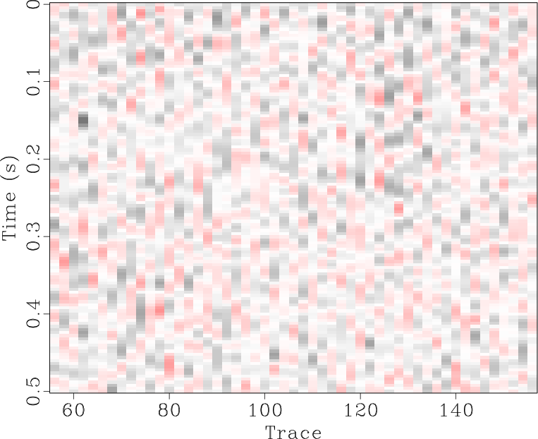
We will perform this application on a 2D field dataset shown in Figure 4a with the aim of separating coherent seismic signals from random noise. We will compare the results of non-stationary local signal-and-noise orthogonalization using the line-search method of Greer and Fomel (2018) and the proposed Gauss-Newton method to obtain the non-stationary triangle smoothing constraint. The initial estimates of signal and noise displayed in Figures 6a and 6d respectively are obtained using the traditional f-x predictive filtering method (Canales, 1984). The non-stationary smoothing radii obtained using 5 iterations of the line-search method and 5 iterations of the proposed method are displayed in Figures 5a and 5b respectively. For the proposed method, we directly substitute the raw field data as
.
To obtain
, Chen and Fomel (2021) propose using the iterative radius estimation approach of Greer and Fomel (2018).
The approach of Greer and Fomel (2018) is based on an optimization problem solved by a line-search method that aims to minimize the difference in local frequency between the low-pass filtered seismic data and the seismic data smoothed via a non-stationary triangle smoothing operator.
We will perform this application on a 2D field dataset shown in Figure 4a with the aim of separating coherent seismic signals from random noise. We will compare the results of non-stationary local signal-and-noise orthogonalization using the line-search method of Greer and Fomel (2018) and the proposed Gauss-Newton method to obtain the non-stationary triangle smoothing constraint. The initial estimates of signal and noise displayed in Figures 6a and 6d respectively are obtained using the traditional f-x predictive filtering method (Canales, 1984). The non-stationary smoothing radii obtained using 5 iterations of the line-search method and 5 iterations of the proposed method are displayed in Figures 5a and 5b respectively. For the proposed method, we directly substitute the raw field data as
 and the 20 Hz low-pass filtered data as
 in equation 15 without accounting for local frequency. In this example, bypassing the local frequency calculation step makes the proposed Gauss-Newton method faster than the line-search method by a factor of 72.
|
|---|
|
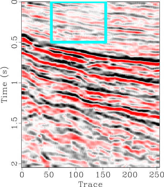
f2-1,f2-z1
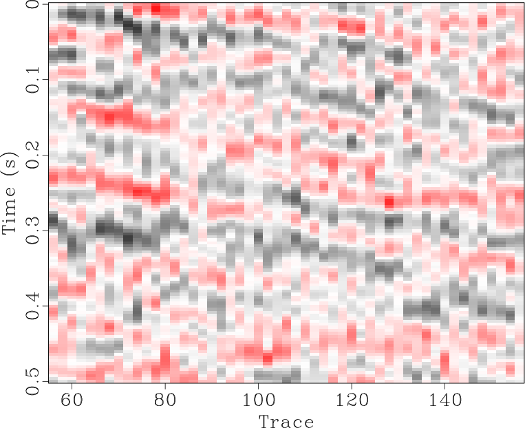
Figure 4. Field data example 1. (a) Raw Field Data. (b) Magnified section. |
|
|
|
|---|
|
rect50,new_rect50
Figure 5. Field data example 1. Estimated non-stationary smoothing radius using 5 iterations of (a) the line-search approach proposed by Chen and Fomel (2021) and (b) the proposed Gauss-Newton approach. |
|
|
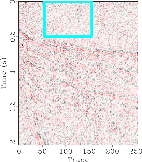
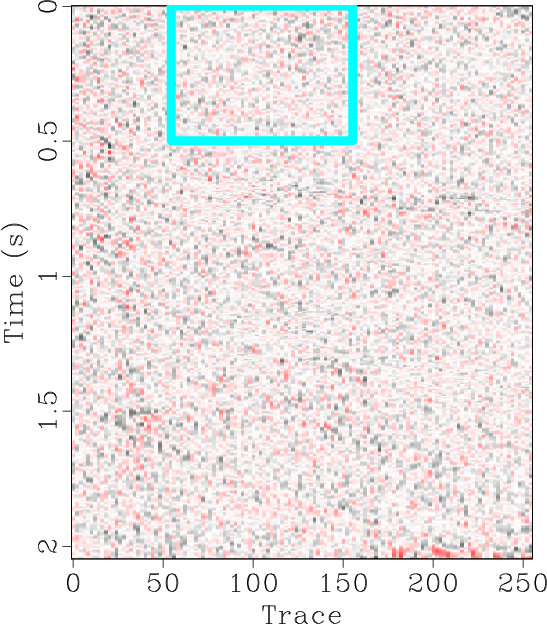
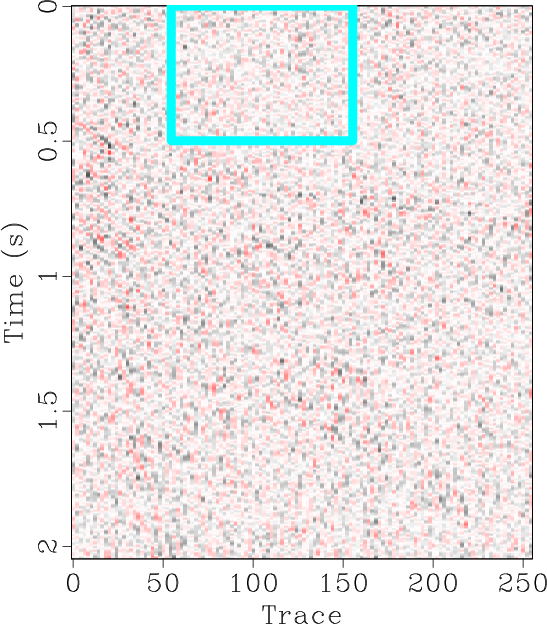
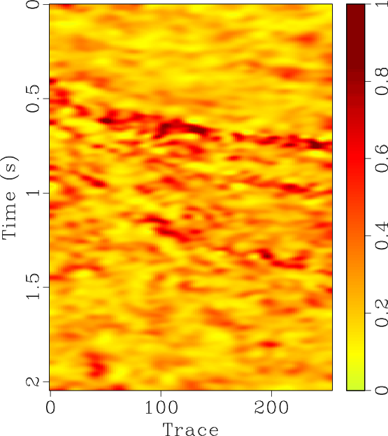
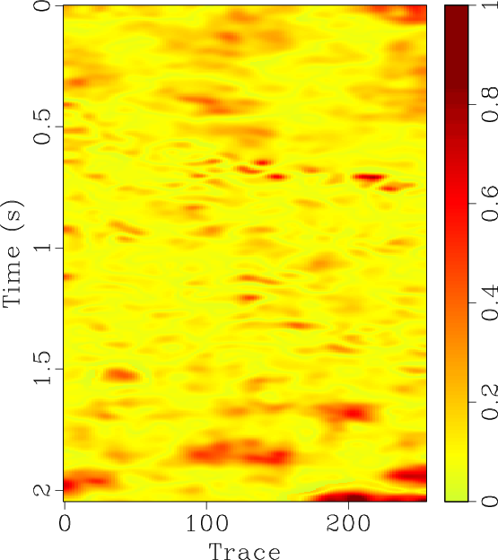
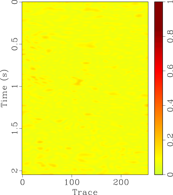
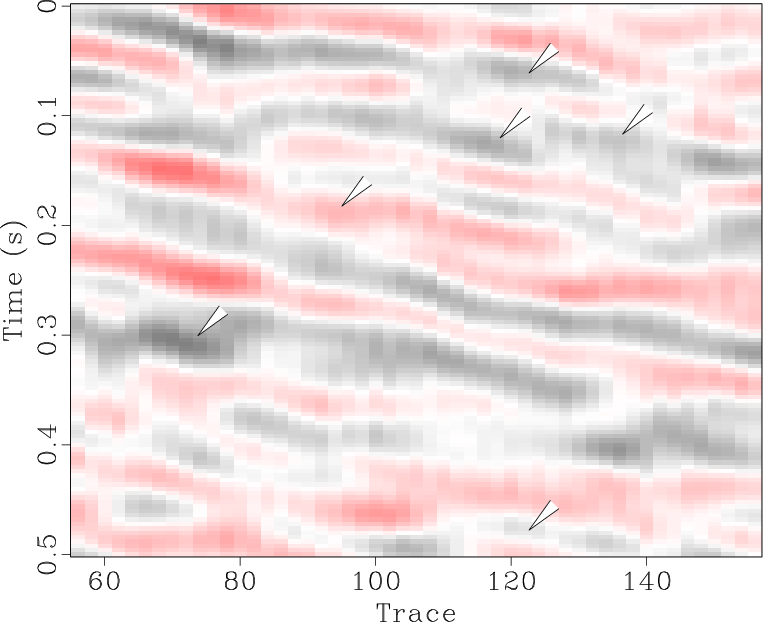
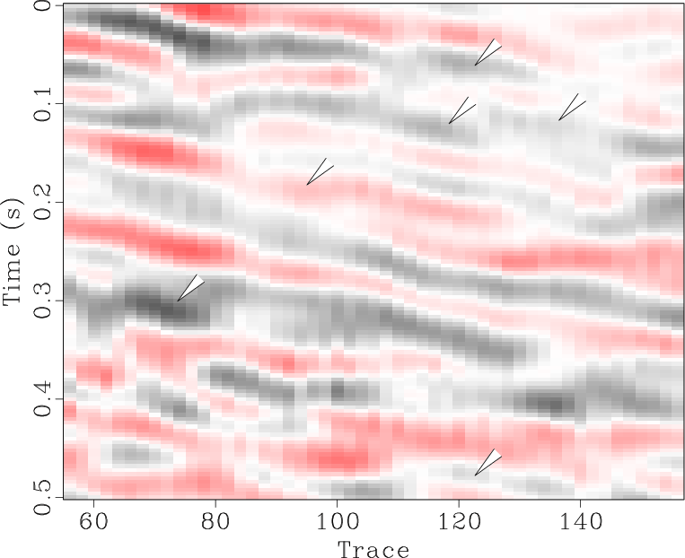
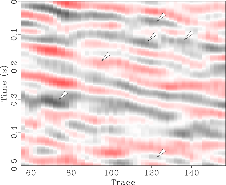
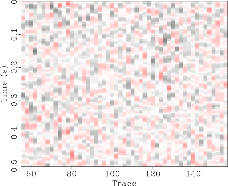
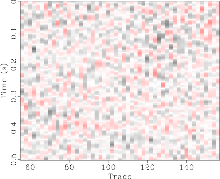
The locally orthogonalized signal and noise using the line-search radius are shown in Figures 6b and 6e respectively, and the locally orthogonalized signal and noise using the Gauss-Newton radius are shown in Figures 6c and 6f respectively. The local similarity is a metric that can be used to evaluate signal and noise separation (Chen and Fomel, 2015). The local similarity between the signal and noise using the f-x method, non-stationary orthogonalization using the line-search radius, and non-stationary orthogonalization using the Gauss-Newton radius is displayed in Figures 7a, 7b, and 7c respectively. The proposed method does the best job of separating coherent signals from random noise since its corresponding local similarity values are the smallest. The zoomed in results of signal and noise separation for the three methods are displayed in Figure 8. In the zoomed in signals, we point to the areas where the signal is stronger for non-stationary orthogonalization using the proposed Gauss-Newton method compared to the two other approaches. In the zoomed in noise results, these same areas correspond to locations of higher signal leakage for the two other methods compared to the proposed method. Thus, from a visual standpoint, the proposed method recovers the strongest signals and also achieves the least signal leakage in the removed noise.
|
|---|
|
f2-fx-1,f2-orthon-1,new-f2-orthon-1,f2-fx-1-n,f2-orthon-1-n,new-f2-orthon-1-n
Figure 6. Field data example 1. De-noised data using the (a) f-x method, (b) non-stationary orthogonalization using line-search radius proposed by Chen and Fomel (2021) for regularization, and (c) non-stationary orthogonalization using proposed Gauss-Newton radius for regularization. (d-f) Removed noise corresponding to (a-c), respectively. |
|
|
|
|---|
|
f2-s,f2-s-orthon,new-f2-s-orthon
Figure 7. Field data example 1. Local similarity of de-noised data and removed noise for (a) f-x method, (b) non-stationary orthogonalization using the line-search radius proposed by Chen and Fomel (2021), and (c) non-stationary orthogonalization using the proposed Gauss-Newton radius. |
|
|
|
|---|
|
f2-fx-z1-0,f2-orthon-z1-0,new-f2-orthon-z1-0,f2-fx-z1-n,f2-orthon-z1-n,new-f2-orthon-z1-n
Figure 8. Field data example 1. (a-f) Magnified sections corresponding to framed boxes in Figure 6 (a-f) respectively. |
|
|
|
|
|
|
Least-squares non-stationary triangle smoothing |
![$\displaystyle \mathbf{w} = [\lambda^2 \mathbf{I} + \mathbf{T} (\mathbf{S}^T\mathbf{S} -\lambda^2 \mathbf{I})]^{-1}\mathbf{T}\mathbf{S}^T\mathbf{n},$](img52.png)