|
|
|
|
Least-squares non-stationary triangle smoothing |
Next: Conclusions Up: Applications Previous: Non-stationary local slope estimation
|
|
|
|
Least-squares non-stationary triangle smoothing |
|
|---|
|
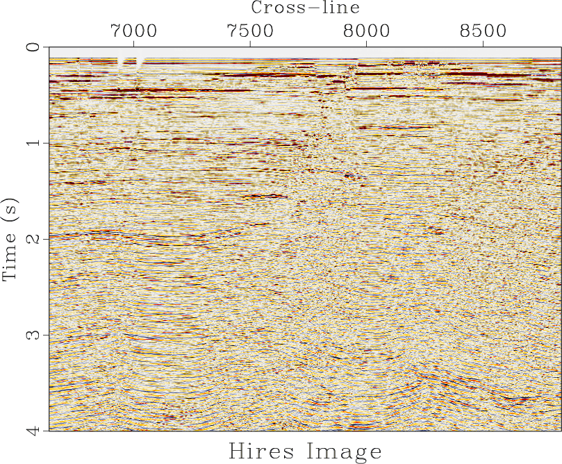
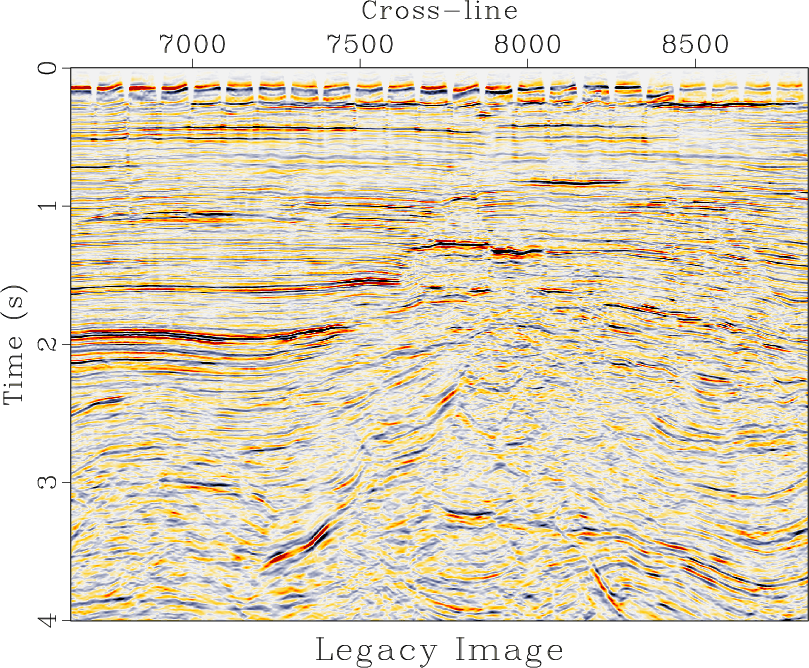
hires,legacy
Figure 11. Field data example 3. (a) High-resolution image. (b) Low-resolution legacy image. |
|
|
We match the two datasets using the proposed radius estimation method substituting the high-resolution data as
 , and the low-resolution data as
 in equation 15.
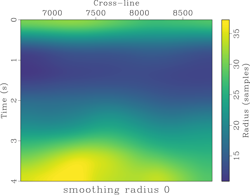
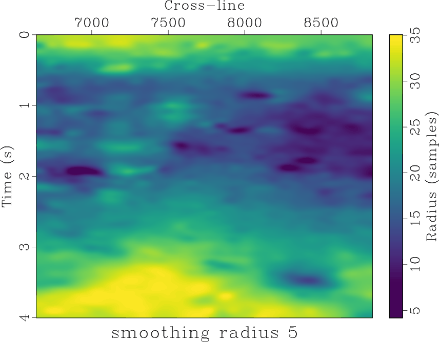
The starting model for the radius is chosen carefully to preserve stability. The initial guess for the radius displayed in Figure 12a is a smooth version of the theoretical radius proposed by Greer and Fomel (2018). The radius estimated after 5 iterations is displayed in Figure 12b.
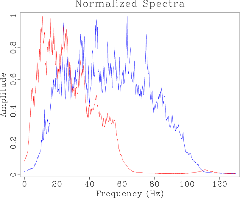
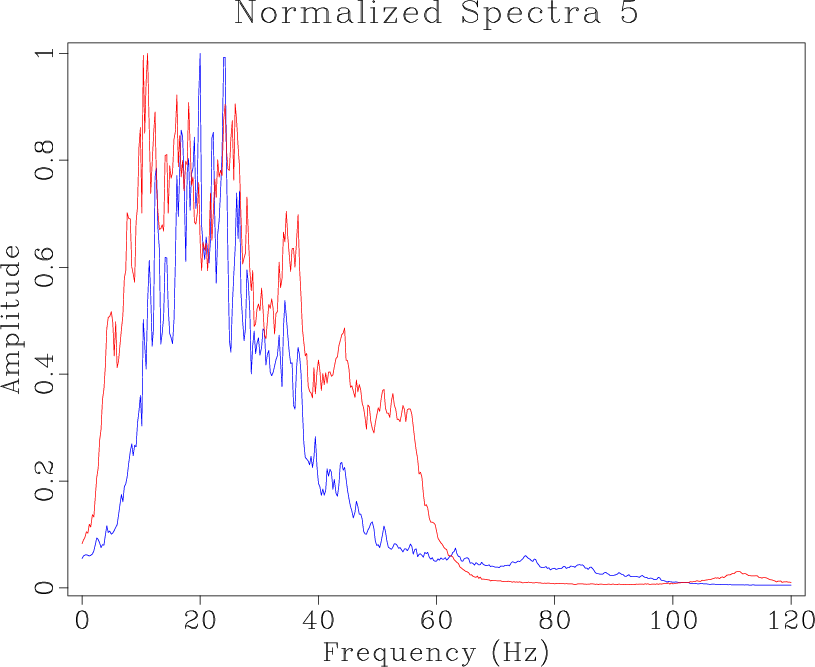
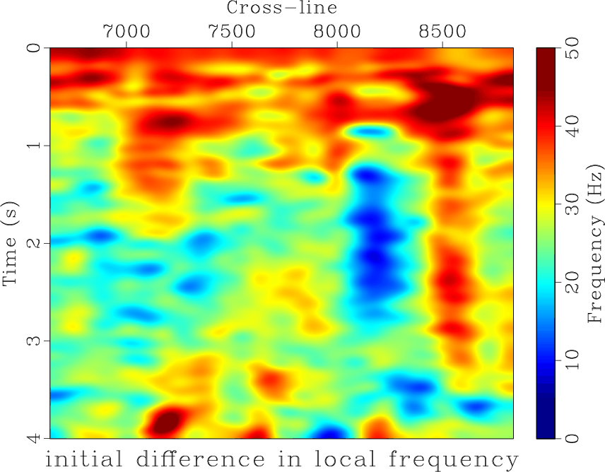
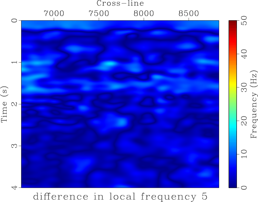
The spectral content of the two datasets before and after non-stationary smoothing is displayed in Figure 13, and the differences in local frequency between the two datasets before and after non-stationary smoothing is displayed in Figure 14.
The results indicate that the frequency content between the two datasets is better balanced after smoothing with the newly estimated radius.
in equation 15.
The starting model for the radius is chosen carefully to preserve stability. The initial guess for the radius displayed in Figure 12a is a smooth version of the theoretical radius proposed by Greer and Fomel (2018). The radius estimated after 5 iterations is displayed in Figure 12b.
The spectral content of the two datasets before and after non-stationary smoothing is displayed in Figure 13, and the differences in local frequency between the two datasets before and after non-stationary smoothing is displayed in Figure 14.
The results indicate that the frequency content between the two datasets is better balanced after smoothing with the newly estimated radius.
|
|---|
|
rect00,rectn50
Figure 12. Field data example 3. (a) The initial guess for the smoothing radius, a smoothed version of the theoretical radius proposed by Greer and Fomel (2018). (b) Estimated smoothing radius using 5 iterations of the proposed Gauss-Newton method matching the high-resolution data and the 18 Hz high-pass filtered low-resolution data. |
|
|
|
|---|
|
nspectra,hires-smooth50-spec
Figure 13. Field data example 3. Normalized spectra of low-resolution legacy data (red) and high-resolution data (blue) (a) before and (b) after 18 Hz high-pass filtering of low-resolution legacy data and non-stationary smoothing of high-resolution data. |
|
|
|
|---|
|
freqdif,locfreqdif50
Figure 14. Field data example 3. (a) Initial difference in local frequency between low-resolution legacy data and high-resolution data. (b) Difference in local frequency between 18 Hz high-pass filtered low-resolution legacy data and non-stationary triangle-smoothed high-resolution data. |
|
|
|
|
|
|
Least-squares non-stationary triangle smoothing |