|
|
|
|
Effects of lateral heterogeneity on time-domain processing parameters |
Next: Appendix D Possible extension Up: Sripanich et al.: Effects Previous: Multi-layer case
|
|
|
|
Effects of lateral heterogeneity on time-domain processing parameters |
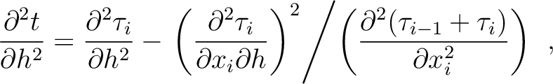
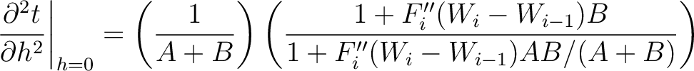
As opposed to the exact recursion proposed in this study, a simpler summation scheme was previously used to accumulate the effects from heterogeneity. A review of this concept can be found in Blias (2006) and we briefly summarize the essentials here. One way to interpret this summation process is to examine one interface at a time and assume that apart from the considered interface, other intermediate layers between the source at larger depth and the receiver at the surface are laterally homogeneous (1D). Under this assumption, one can evaluate the contribution from lateral heterogeneity for this particular interface and its two adjacent layers using the result from the two-layer case (equation (43)). To further describe this process, we first assume that all sublayers are homogeneous isotropic similarly to what was done by Blias and consider only one non-flat interface at  -th. Therefore, we have
 and
and
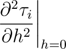
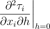
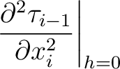
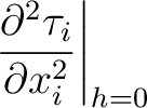
 denote the effective time below and above the non-flat -th interface. To evaluate pertaining derivatives, we use equation (15) for general media in the main text and focus only on the effects from curved interfaces at the moment by setting
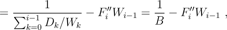
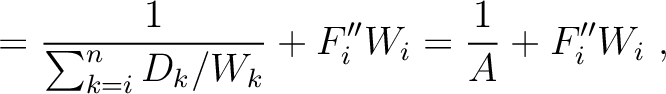
 to exclude the effects from lateral velocity variations. Subsequently, we can derive the following expressions:
where
to exclude the effects from lateral velocity variations. Subsequently, we can derive the following expressions:
where  is the slowness for each isotropic sublayer
  and
and  is its thickness. We also introduce dummy variables
  and
and  to facilitate subsequent derivation. Substituting equation (56) into equation (55) leads to
where
to facilitate subsequent derivation. Substituting equation (56) into equation (55) leads to
where
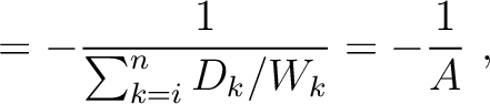
 with
with  being the total one-way zero-offset traveltime in the 1D medium and
  being the corresponding root-mean-square velocity. Therefore, the first term on the right-hand side of equation (57) represents the usual second-order one-way traveltime derivative at zero offset in the 1D medium, whereas the second term is the contribution from lateral heterogeneity. When
  for flat -th interface, this second term becomes unity.
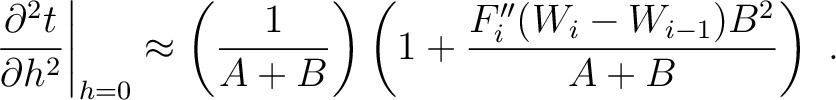
To further simplify equation (57), it can be linearized with respect to  , which results in
rather than being computed through a recursive evaluation as proposed in this study. Equation (58) is similar to equation 5 in Blias (2009b). For the effects from lateral velocity change ( ), a similar derivation procedure can be adopted. Finally, we emphasize that due to the steps taken in the derivation of equation (58), the terms involving
  apparent in the general expressions in equation (15) are missing. These terms are also absent from the final result shown in equation 1 of Blias (2009b).
|
|
|
|
Effects of lateral heterogeneity on time-domain processing parameters |