Layered isotropic model with velocity gradient

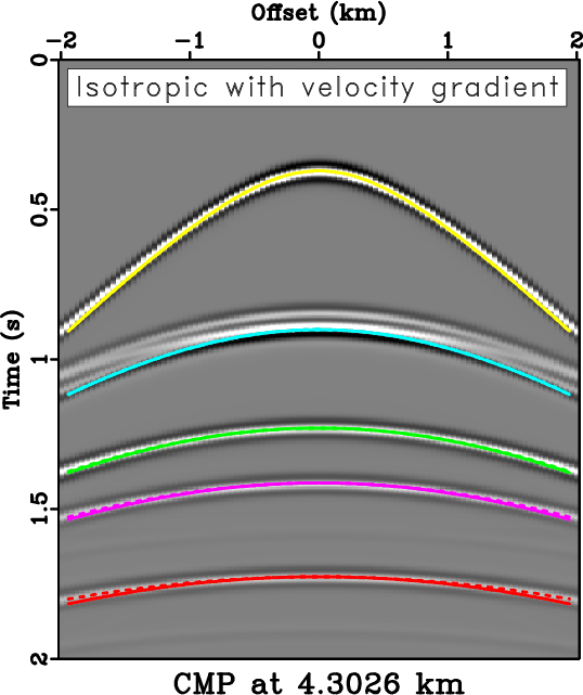
Next, we test the proposed framework in a layered isotropic model with a constant horizontal velocity gradient in each sublayer (equation 19). The model structure is similar to the previous case (Figure 4) and the model parameters are given in Table 2. In this example, both effects from the curved reflectors (derivatives of $F$) and the laterally varying slowness (derivatives of $W$) are important. 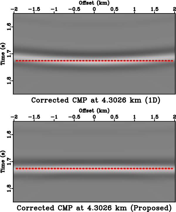Figure 6 shows the CMP gather at 4.3 $km$ that compares the predicted moveout curves based on the 1-D assumption with those from the proposed framework that honor the effects of heterogeneity. We can again observe an improved flatness of moveout-corrected gather from the latter.

hypercompare2,warpedcompare2
Figure 6. (a) An example CMP gather from the layered isotropic model at 4.3 $km$. Note the multiple reflection events above the second moveout curve that are caused by the syncline. The solid lines correspond to regular moveout predictions based on the assumption of 1-D stratified model, whereas the dashed lines correspond to those from the proposed framework that takes into account the effects from heterogeneity. (b) Flattened reflections from the bottom interface using the NMO velocity with 1-D assumption (top) and the proposed framework (bottom). We can clearly observed improved flatness from using the proposed framework.

	$v$ $(km/s)$	Gradient $(1/s)$
Layer 1	2.50	-0.06
Layer 2	3.20	0.15
Layer 3	3.40	0.20
Layer 4	3.70	0.30
Layer 5	3.86	0.35

Table 2. Model parameters for the layered isotropic model. The reference velocity at 3 $km$ and horizontal velocity gradient.