|
|
|
|
Effects of lateral heterogeneity on time-domain processing parameters |
Next: Reflection traveltime in multilayer Up: Numerical examples Previous: Numerical examples
|
|
|
|
Effects of lateral heterogeneity on time-domain processing parameters |
 is the horizontal velocity gradient. In this medium, the two-point traveltime of a ray between the source at (
 ,
, ) and the receiver at (
 ,
, ) can be computed analytically from
The exact second-order derivative of traveltime can then be found by twice differentiating equation 20 with respect to
) can be computed analytically from
The exact second-order derivative of traveltime can then be found by twice differentiating equation 20 with respect to  .
.
We randomly generate 10,000 models from uniform distributions defined with the following parameter ranges:
 |
 |
(21) |
 |
 |
|
 |
 |
|
 |
 |
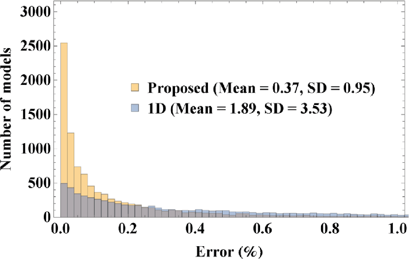
 . Figure 2 shows a comparison of histograms for the relative errors of both methods with respect to the analytical results. We can observe that the results from the proposed approach (equation 17) as depicted by the orange histogram has higher peaks at low error levels than that of the overlaid blue histogram associated with the results from the 1-D approach. In other words, the proposed approach can lead to a small level of prediction error in a larger proportion of the generated models. The mean, the standard deviation, and the maximum error from the proposed approach are 0.37, 0.95 and 4.28 per cent in comparison with 1.89, 3.53 and 12.78 per cent from the usual 1-D computation. These results suggest a better performance from the proposed approach and corroborate our theoretical findings.
|
|---|
|
fig2
Figure 2. A comparison of error histograms from 10 000 randomly generated models for the results from 1-D computations (Blue) and those from the proposed method (Orange) according to equation 17 in the single layer case with both vertical and horizontal velocity variations. We can observe relatively smaller errors in a larger proportion of the models from the latter, which corroborate our theoretical findings. |
|
|
For an additional example, we consider a similar setup with only horizontal velocity gradient ( ), which leads to the 1-D traveltime derivative simply being
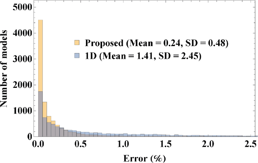
. The result of this experiment is shown in Figure 3 with the mean, the standard deviation, and the maximum error from the proposed approach equal to 0.24, 0.48 and 4.28 per cent in comparison with 1.41, 2.45 and 17.58 per cent from the usual 1-D computation. An analogous conclusion to the previous case can be drawn.
), which leads to the 1-D traveltime derivative simply being
. The result of this experiment is shown in Figure 3 with the mean, the standard deviation, and the maximum error from the proposed approach equal to 0.24, 0.48 and 4.28 per cent in comparison with 1.41, 2.45 and 17.58 per cent from the usual 1-D computation. An analogous conclusion to the previous case can be drawn.
|
|---|
|
fig3
Figure 3. A comparison of error histograms from 10 000 randomly generated models for the results from 1-D computations (Blue) and those from the proposed method (Orange) according to equation 17 in the single layer case with only horizontal velocity variation. We can observe relatively smaller errors in a larger proportion of the models from the latter, which corroborate our theoretical findings. |
|
|
|
|
|
|
Effects of lateral heterogeneity on time-domain processing parameters |

![$\displaystyle t(x,z) = \frac{1}{g_x} \mathrm{arccosh} \left(1+ \frac{g^2_x~[(x-x_0)^2+(z-z_0)^2]}{2v(x)v_0} \right)~.$](img118.png)