|
 |
 |
 | Theory of differential offset continuation |  |
![[pdf]](icons/pdf.png) |
Next: About this document ...
Up: Theory of differential offset
Previous: Acknowledgments
-
Babich, V. M., 1991, Short-wavelength diffraction theory: asymptotic
methods: Springer-Verlag.
-
-
Bagaini, C., and U. Spagnolini, 1993, Common shot velocity analysis by shot
continuation operator: 63rd Ann. Internat. Mtg, Soc. of Expl. Geophys.,
673-676.
-
-
----, 1996, 2-D continuation operators and their applications:
Geophysics, 61, 1846-1858.
-
-
Bale, R., and H. Jakubowicz, 1987, Post-stack prestack migration: 57th Ann.
Internat. Mtg, Soc. of Expl. Geophys., Session:S14.1.
-
-
Beylkin, G., 1985, Imaging of discontinuities in the inverse scattering
problem by inversion of a causal generalized Radon transform: Journal of
Mathematical Physics, 26, 99-108.
-
-
Biondi, B., and N. Chemingui, 1994, Transformation of 3-D prestack data by
azimuth moveout (AmO): 64th Ann. Internat. Mtg, Soc. of Expl. Geophys.,
1541-1544.
-
-
Biondi, B., S. Fomel, and N. Chemingui, 1998, Azimuth moveout for 3-D
prestack imaging: Geophysics, 63, 574-588.
-
-
Black, J. L., K. L. Schleicher, and L. Zhang, 1993, True-amplitude imaging and
dip moveout: Geophysics, 58, 47-66.
-
-
Bleistein, N., 1984, Mathematical methods for wave phenomena: Academic Press
Inc. (Harcourt Brace Jovanovich Publishers).
-
-
----, 1990, Born DMO revisited, in 60th Annual Internat. Mtg.,
Soc. Expl. Geophys., Expanded Abstracts: Soc. Expl. Geophys., 1366-1369.
-
-
Bleistein, N., and H. H. Jaramillo, 2000, A platform for Kirchhoff data
mapping in sealer models of data acquisition: Geophys. Prosp., 48,
135-162.
-
-
Bleistein, N., J. W. Stockwell, and J. K. Cohen, 2001, Mathematics of
multidimensional seismic imaging, migration, and inversion: Springer Verlag.
-
-
Bolondi, G., E. Loinger, and F. Rocca, 1982, Offset continuation of seismic
sections: Geophys. Prosp., 30, 813-828.
-
-
Canning, A., and G. H. F. Gardner, 1996, Regularizing 3-D data sets with
DmO: Geophysics, 61, 1103-1114.
- (Discussion and reply in GEO-62-4-1331).
-
Chemingui, N., and B. Biondi, 1996, Handling the irregular geometry in
wide-azimuth surveys: 66th Ann. Internat. Mtg, Soc. of Expl. Geophys.,
32-35.
-
-
Claerbout, J. F., 1976, Fundamentals of geophysical data processing:
Blackwell.
-
-
Courant, R., 1962, Methods of mathematical physics: Interscience Publishers.
-
-
Deregowski, S. M., and F. Rocca, 1981, Geometrical optics and wave theory of
constant offset sections in layered media: Geophys. Prosp., 29,
374-406.
-
-
Fomel, S., 2001, Three-dimensional seismic data regularization: PhD thesis,
Stanford University.
-
-
----, 2003a, Asymptotic pseudounitary stacking operators: Geophysics, 68, 1032-1042.
-
-
----, 2003b, Seismic reflection data interpolation with differential offset
and shot continuation: Geophysics, 68, 733-744.
-
-
Fomel, S., and N. Bleistein, 2001, Amplitude preservation for offset
continuation: Confirmation for Kirchhoff data: Journal of Seismic
Exploration, 10, 121-130.
-
-
Fomel, S., N. Bleistein, H. Jaramillo, and J. K. Cohen, 1996, True amplitude
DmO, offset continuation and AvA/AvO for curved reflectors: 66th
Ann. Internat. Mtg, Soc. of Expl. Geophys., 1731-1734.
-
-
Fomel, S. B., 1994, Kinematically equivalent differential operator for offset
continuation of seismic sections: Russian Geology and Geophysics, 35,
122-134.
-
-
Fomel, S. B., and B. L. Biondi, 1995, The time and space formulation of
azimuth moveout: 65th Ann. Internat. Mtg, Soc. of Expl. Geophys., 1449-1452.
-
-
Gazdag, J., 1978, Wave equation migration with the phase-shift method:
Geophysics, 43, 1342-1351.
-
-
Goldin, S., 1990, A geometric approach to seismic processing: the method of
discontinuities, in SEP-67: Stanford Exploration Project, 171-210.
-
-
Goldin, S. V., 1988, Transformation and recovery of discontinuities in
problems of tomographic type: Institute of Geology and Geophysics.
-
-
----, 1994, Superposition and continuation of tranformations used in
seismic migration: Russian Geology and Geophysics, 35, 131-145.
-
-
Goldin, S. V., and S. B. Fomel, 1995, Estimation of reflection coefficient in
DMO: Russian Geology and Geophysics, 36, 103-115.
-
-
Gradshtein, I. S., and I. M. Ryzhik, 1994, Table of integrals, series, and
products: Boston: Academic Press.
-
-
Haddon, R. A. W., and P. W. Buchen, 1981, Use of Kirchhoff's formula for
body wave calculations in the earth: Geophys. J. Roy. Astr. Soc., 67,
587-598.
-
-
Hale, D., 1984, Dip-moveout by Fourier transform: Geophysics, 49,
741-757.
-
-
----, 1991, Course notes: Dip moveout processing: Soc. Expl. Geophys.
-
-
----, 1995, DMo Processing, in DMO processing: Soc. of Expl.
Geophys., 496.
- (Reprints).
-
Hale, I. D., 1983, Dip moveout by Fourier transform: PhD thesis, Stanford
University.
-
-
Hill, S. J., R. Stolt, and S. Chiu, 2001, Altering offsets and azimuths: The
Leading Edge, 20, 210-213.
-
-
Liner, C., 1990, General theory and comparative anatomy of dip moveout:
Geophysics, 55, 595-607.
-
-
Liner, C. L., 1991, Born theory of wave-equation dip moveout: Geophysics, 56, 182-189.
-
-
Liner, C. L., and J. K. Cohen, 1988, An amplitude-preserving inverse of hale`s
DmO: 58th Ann. Internat. Mtg, Soc. of Expl. Geophys., Session:S17.5.
-
-
Notfors, C. D., and R. J. Godfrey, 1987, Dip moveout in the
frequency-wavenumber domain (short note): Geophysics, 52, 1718-1721.
-
-
Petkovsek, M., H. S. Wilf, and D. Zeilberger, 1996,
 : A K Peters Ltd.
-
-
Ronen, J., 1987, Wave equation trace interpolation: Geophysics, 52,
973-984.
-
-
Ronen, S., 1994, Handling irregular geometry: Equalized DmO and beyond:
64th Ann. Internat. Mtg, Soc. of Expl. Geophys., 1545-1548.
-
-
Ronen, S., V. Sorin, and R. Bale, 1991, Spatial dealiasing of 3-D seismic
reflection data: Geophysical Journal International, 503-511.
-
-
Stolt, R. H., 1978, Migration by Fourier transform: Geophysics, 43,
23-48.
- (Discussion and reply in GEO-60-5-1583).
-
Stovas, A. M., and S. B. Fomel, 1996, Kinematically equivalent integral DMO
operators: Russian Geology and Geophysics, 37, 102-113.
-
-
Tenenbaum, M., and H. Pollard, 1985, Ordinary differential equations : an
elementary textbook for students of mathematics, engineering, and the
sciences: Dover Publications.
-
-
Cervený, V., 2001, Seismic ray theory: Cambridge University Press.
-
-
Watson, G. N., 1952, A treatise on the theory of Bessel functions, 2nd ed.:
Cambridge University Press.
-
-
Zhou, B., I. M. Mason, and S. A. Greenhalgh, 1996, An accurate formulation of
log-stretch dip moveout in the frequency-wavenumber domain: Geophysics, 61, 815-820.
-
Appendix
A
Second-order reflection traveltime derivatives
This appendix contains a derivation of equations connecting
second-order partial derivatives of the reflection traveltime with the
geometric properties of the reflector in a constant velocity medium.
These equations are used in the main text of this paper to describe
the amplitude behavior of offset continuation. Let  be the
reflection traveltime from the source
be the
reflection traveltime from the source  to the receiver
  .
Consider a formal equality
.
Consider a formal equality
 |
(114) |
where  is the reflection point parameter,
  corresponds to the
incident ray, and
corresponds to the
incident ray, and  corresponds to the reflected ray.
Differentiating (A-1) with respect to and yields
corresponds to the reflected ray.
Differentiating (A-1) with respect to and yields
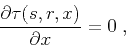
According to Fermat's principle, the two-point reflection ray path must
correspond to the traveltime stationary point. Therefore
 |
(117) |
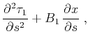
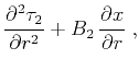
for any and . Taking into account (A-4) while
differentiating (A-2) and (A-3), we get
where
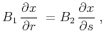
Differentiating equation (A-4) gives us the additional
pair of equations
where
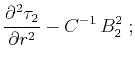
Solving the system (A-8) - (A-9) for
 and
and
 and substituting
the result into (A-5) - (A-7) produces the
following set of expressions:
and substituting
the result into (A-5) - (A-7) produces the
following set of expressions:
In the case of a constant velocity medium, expressions (A-10) to
(A-12) can be applied directly to the explicit
equation for the two-point eikonal
 |
(126) |
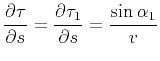
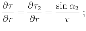
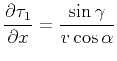
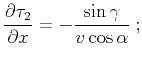
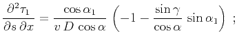
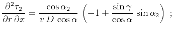
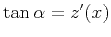
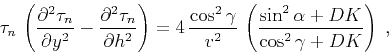
Differentiating (A-13) and taking into account the trigonometric
relationships for the incident and reflected rays (Figure
1), one can
evaluate all the quantities in (A-10) to (A-12) explicitly.
After some heavy algebra, the resultant expressions for the traveltime
derivatives take the form
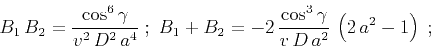 |
(131) |
 |
(132) |
 |
(133) |
Here  is the length of the normal (central) ray,
  is its dip angle
(
is its dip angle
(
 ,
,
 ),
),
 is the reflection angle
 ,
,  is the reflector
curvature at the reflection point
is the reflector
curvature at the reflection point
 , and
, and
 is the dimensionless function of and defined in (47).
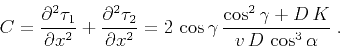
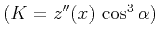
The equations derived in this appendix were used to obtain the equation
 |
(134) |
which coincides with (50) in the main text.
Appendix
B
The kinematics of offset continuation
This Appendix presents an alternative method to derive equation
(70), which describes the summation path of the
integral offset continuation operator. The method is based on the
following considerations.
The summation path of an integral (stacking) operator coincides with
the phase function of the impulse response of the inverse operator.
Impulse response is by definition the operator reaction to an impulse
in the input data. For the case of offset continuation, the input is a
reflection common-offset gather. From the physical point of view, an
impulse in this type of data corresponds to the special focusing
reflector (elliptical isochrone) at the depth. Therefore, reflection
from this reflector at a different constant offset corresponds to the
impulse response of the OC operator. In other words, we can view
offset continuation as the result of cascading prestack common-offset
migration, which produces the elliptic surface, and common-offset
modeling (inverse migration) for different offsets. This approach
resemble that of Deregowski and Rocca (1981). It was also applied to a
more general case of azimuth moveout (AMO) by
Fomel and Biondi (1995) and fully generalized by
Bleistein and Jaramillo (2000). The geometric approach implies that
in order to find the summation pass of the OC operator, one should
solve the kinematic problem of reflection from an elliptic reflector
whose focuses are in the shot and receiver locations of the output
seismic gather.
In order to solve this problem , let us consider an elliptic surface of
the general form
 |
(135) |
where  . In a constant velocity medium, the reflection
ray path for a given source-receiver pair on the surface is controlled
by the position of the reflection point . Fermat's principle
provides a required constraint for finding this position. According to
Fermat's principle, the reflection ray path corresponds to a
stationary value of the travel-time. Therefore, in the neighborhood of
this path,
. In a constant velocity medium, the reflection
ray path for a given source-receiver pair on the surface is controlled
by the position of the reflection point . Fermat's principle
provides a required constraint for finding this position. According to
Fermat's principle, the reflection ray path corresponds to a
stationary value of the travel-time. Therefore, in the neighborhood of
this path,
 |
(136) |
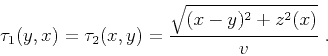
where and stand for the source and receiver locations on the
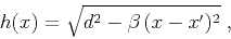
surface, and  is the reflection traveltime
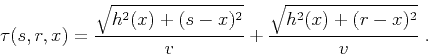 |
(137) |
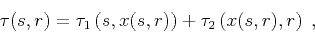
Substituting equations (B-3) and (B-1) into
(B-2) leads to a quadratic algebraic equation on the
reflection point parameter . This equation has the explicit
solution
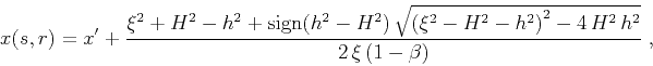 |
(138) |
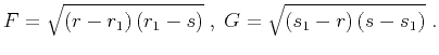
where  ,
,  ,
,  , and
, and
 . Replacing in equation
(B-3) with its expression (B-4) solves
the kinematic part of the problem, producing the explicit traveltime
expression
. Replacing in equation
(B-3) with its expression (B-4) solves
the kinematic part of the problem, producing the explicit traveltime
expression
 |
(139) |
where
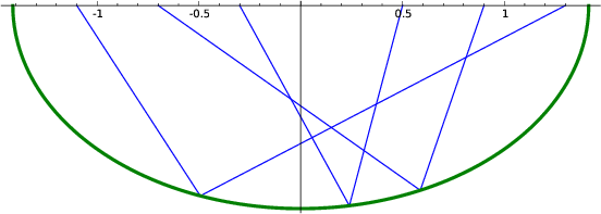
The two branches of equation (B-5) correspond to the
difference in the geometry of the reflected rays in two different
situations. When a source-and-receiver pair is inside the focuses of
the elliptic reflector, the midpoint  and the reflection point
are on the same side of the ellipse with respect to its small
semi-axis. They are on different sides in the opposite case (Figure
B-1).
and the reflection point
are on the same side of the ellipse with respect to its small
semi-axis. They are on different sides in the opposite case (Figure
B-1).
Reflections from an ellipse. The three pairs of reflected rays
correspond to a common midpoint (at 0.1) and different offsets. The
focuses of the ellipse are at 1 and -1.
If we apply the NMO correction, equation (B-5) is transformed to
 |
(140) |
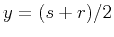
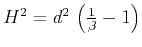
Then, recalling the relationships between the parameters of the
focusing ellipse ,  and
and  and the parameters of the
output seismic gather (Deregowski and Rocca, 1981)
and the parameters of the
output seismic gather (Deregowski and Rocca, 1981)
 |
(141) |
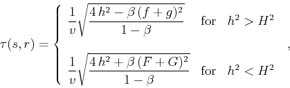
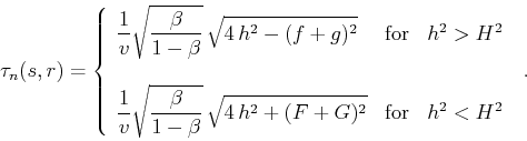
and substituting expressions (B-7) into equation (B-6) yields the
expression
 |
(142) |
where
It is easy to verify algebraically the mathematical equivalence of
equation (B-8) and equation (70) in the
main text. The kinematic approach described in this appendix applies
equally well to different acquisition configurations of the input and
output data. The source-receiver parameterization used in
(B-8) is the actual definition for the summation path of
the integral shot continuation operator
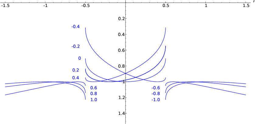
(Bagaini and Spagnolini, 1996,1993). A family of these summation
curves is shown in Figure B-2.
Summation paths of the integral shot continuation. The output source
is at -0.5 km. The output receiver is at 0.5 km. The indexes of the
curves correspond to the input source location.
|
|
|
|
| Theory of differential offset continuation | |
|
Next: About this document ...
Up: Theory of differential offset
Previous: Acknowledgments
2014-03-26