|
|
|
|
Preconditioning |
Jon Claerbout
In Chapter ![]() , we developed adjoints and
in Chapter
, we developed adjoints and
in Chapter ![]() , we developed inverse operators.
Logically, correct solutions come only through inversion.
Real life, however, seems nearly the opposite.
This situation is puzzling but intriguing.
It seems an easy path to fame and profit would
be to go beyond adjoints by introducing
some steps of inversion.
It is not that easy.
Images contain so many unknowns.
Mostly, we cannot iterate to completion
and need concern ourselves with the rate of convergence.
Often, necessity limits us to a handful
of iterations whereby in principle,
millions or billions are required.
, we developed inverse operators.
Logically, correct solutions come only through inversion.
Real life, however, seems nearly the opposite.
This situation is puzzling but intriguing.
It seems an easy path to fame and profit would
be to go beyond adjoints by introducing
some steps of inversion.
It is not that easy.
Images contain so many unknowns.
Mostly, we cannot iterate to completion
and need concern ourselves with the rate of convergence.
Often, necessity limits us to a handful
of iterations whereby in principle,
millions or billions are required.
When you fill your car with gasoline, it derives more from an adjoint than an inverse. Industrial seismic data processing relates more to adjoints than to inverses though there is a place for both, of course. It cannot be much different with medical imaging.
First consider cost.
For simplicity, consider a data space with ![]() values
and a model (or image) space of the same size.
The computational cost of applying a dense adjoint
operator increases in direct proportion to the number
of elements in the matrix, in this case
values
and a model (or image) space of the same size.
The computational cost of applying a dense adjoint
operator increases in direct proportion to the number
of elements in the matrix, in this case ![]() .
To achieve the minimum discrepancy between modeled data
and observed data (inversion) theoretically requires
.
To achieve the minimum discrepancy between modeled data
and observed data (inversion) theoretically requires ![]() iterations
raising the cost to
iterations
raising the cost to ![]() .
.
Consider an image of size
![]() .
Continuing, for simplicity, to assume a dense matrix of relations between
model and data,
the cost for the adjoint is
.
Continuing, for simplicity, to assume a dense matrix of relations between
model and data,
the cost for the adjoint is ![]() , whereas, the cost for inversion is
, whereas, the cost for inversion is ![]() .
We consider computational costs for the year 2000, but
noticing that costs go as the sixth power of the mesh size,
the overall situation will not change much in the foreseeable future.
Suppose you give a stiff workout to a powerful machine;
you take an hour to invert a 4,096
.
We consider computational costs for the year 2000, but
noticing that costs go as the sixth power of the mesh size,
the overall situation will not change much in the foreseeable future.
Suppose you give a stiff workout to a powerful machine;
you take an hour to invert a 4,096![]() 4,096 matrix.
The solution, a vector of
4,096 matrix.
The solution, a vector of ![]() components could
be laid into an image of size 64
components could
be laid into an image of size 64 ![]() 64=
64=
![]() = 4,096.
Here is what we are looking at for costs:
= 4,096.
Here is what we are looking at for costs:
| adjoint cost |
|
|
|
|
| inverse cost |
|
|
|
These numbers tell us that for applications with dense operators,
the biggest images that we are likely to see coming from inversion methods
are
![]() , whereas, those from adjoint methods are
, whereas, those from adjoint methods are
![]() .
For comparison, your vision is comparable
to your computer screen at 1,000
.
For comparison, your vision is comparable
to your computer screen at 1,000 ![]() 1,000.
1,000.
|
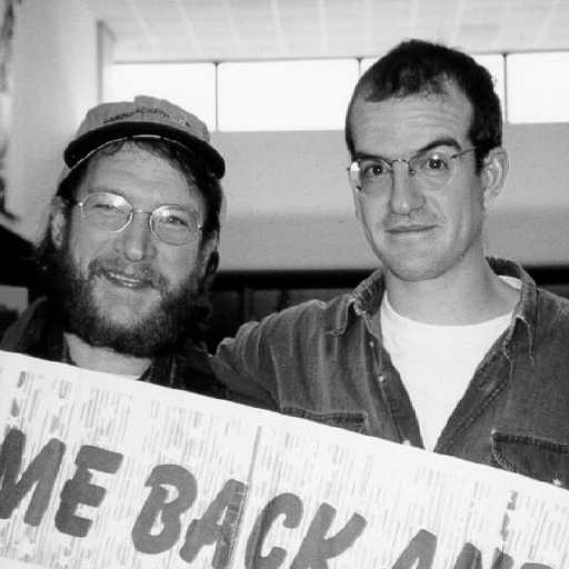
512x512
Figure 1. Jos greets Andrew, ``Welcome back Andrew'' from the Peace Corps. At a resolution of |
|
|---|---|
|
|
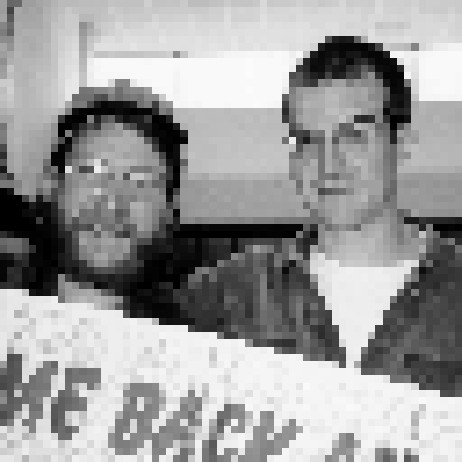
http://sepwww.stanford.edu/sep/jon/family/jos/gifmovie.html holds a movie blinking between Figures 1 and 2.
This cost analysis is oversimplified in that most applications do not require dense operators. With sparse operators, the cost advantage of adjoints is even more pronounced because for adjoints, the cost savings of operator sparseness translate directly to real cost savings. The situation is less favorable and more muddy for inversion. The reason that Chapter 2 covers iterative methods and neglects exact methods is that in practice iterative methods are not run to theoretical completion, but until we run out of patience. But that leaves hanging the question of what percent of theoretically dictated work is actually necessary. If we struggle to accomplish merely one percent of the theoretically required work, can we hope to achieve anything of value?
Cost is a big part of the story, but the story has many other parts. Inversion, while being the only logical path to the best answer, is a path littered with pitfalls. The first pitfall is that the data is rarely able to determine a complete solution reliably. Generally, there are aspects of the image that are not learnable from the data.
|
64x64
Figure 2. Jos greets Andrew, ``Welcome back Andrew'' again. At a resolution of |
|
|---|---|
|
|
When I first realized that practical imaging methods with wide
industrial use amounted merely to the adjoint of forward modeling,
I (and others) thought an easy way to achieve fame and fortune
would be to introduce the first steps toward inversion
along the lines of Chapter ![]() .
Although inversion generally requires a prohibitive number
of steps, I felt that moving in the gradient direction,
the direction of steepest descent, would move us rapidly
in the direction of practical improvements.
This optimism was soon exposed.
Improvements came too slowly.
But then, I learned about the conjugate gradient method that
spectacularly overcomes a well-known speed problem with the
method of steepest descent.
I came to realize it was still too slow.
I learned by watching the convergence in Figure
8,
which led me to the helix method in Chapter 4.
Here we see how it speeds many applications.
.
Although inversion generally requires a prohibitive number
of steps, I felt that moving in the gradient direction,
the direction of steepest descent, would move us rapidly
in the direction of practical improvements.
This optimism was soon exposed.
Improvements came too slowly.
But then, I learned about the conjugate gradient method that
spectacularly overcomes a well-known speed problem with the
method of steepest descent.
I came to realize it was still too slow.
I learned by watching the convergence in Figure
8,
which led me to the helix method in Chapter 4.
Here we see how it speeds many applications.
We also come to understand why the gradient is such a poor direction
both for steepest descent and conjugate gradients.
An indication of our path is found in the contrast between
an exact solution and the gradient.
|
|
|
|
Preconditioning |