Preconditioning

Blocky models

Sometimes, we seek a velocity model that increases smoothly with depth through our scattered measurements of good-quality RMS velocities. Other times, we seek a blocky model. (Where seismic data is poor, a well log could tell us whether or not to choose smooth or blocky.) Here, we see an estimation method that can choose the blocky alternative, or some combination of smooth and blocky.

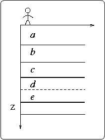
Consider the five-layer model in Figure 6. Each layer has unit traveltime thickness (so integration is simply summation). Let the squared interval velocities be $(a,b,c,d,e)$ with strong reliable reflections at the base of layer $c$ and layer $e$ , and weak, incoherent, ``bad'' reflections at bases of $(a,b,d)$ . Thus, we measure $V_c^2$ the RMS velocity squared of the top three layers and $V_e^2$ for all five layers. Because we have no reflection from at the base of the fourth layer, the velocity in the fourth layer is not measured but a matter for choice. In a smooth linear fit, we would want $d=(c+e)/2$ . In a blocky fit, we would want $d=e$ .

rosales Figure 6. A layered Earth model. The layer interfaces cause reflections. Each layer has a constant velocity in its interior.

Our screen for good reflections looks like $(0,0,1,0,1)$ , and our screen for bad ones looks like the complement $(1,1,0,1,0)$ . We put these screens on the diagonals of diagonal matrices $\bold G$ and $\bold B$ . Our fitting goals are:

$$3V_c^2 \approx a+b+c$$ (36)

$$5V_e^2 \approx a+b+c+d+e$$ (37)

$$u_0 \approx a$$ (38)

$$\approx -a+b$$ 0 (39)

$$\approx -b+c$$ 0 (40)

$$\approx -c+d$$ 0 (41)

$$\approx -d+e$$ 0 (42)

For the blocky solution, we do not want the fitting goal (41). Further explanations await completion of examples.

Preconditioning