Next: SeaBeam
Up: Preconditioning
Previous: INVERSE LINEAR INTERPOLATION
There are at least three ways to fill empty bins.
Two require a roughening operator  while
the third requires a smoothing operator, which
(for comparison purposes) we denote
while
the third requires a smoothing operator, which
(for comparison purposes) we denote
 .
The three methods are generally equivalent
though they differ in significant details.
.
The three methods are generally equivalent
though they differ in significant details.
The original way in
Chapter ![[*]](icons/crossref.png) is to
restore missing data
by ensuring the restored data,
after specified filtering,
has minimum energy, say
is to
restore missing data
by ensuring the restored data,
after specified filtering,
has minimum energy, say
 .
Introduce the selection mask operator
.
Introduce the selection mask operator  ,
a diagonal matrix with
ones on the known data and zeros elsewhere
(on the missing data).
Thus,
,
a diagonal matrix with
ones on the known data and zeros elsewhere
(on the missing data).
Thus,
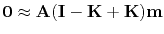 or:
or:
 |
(43) |
where we define  to be the data
with missing values set to zero by
to be the data
with missing values set to zero by
 .
.
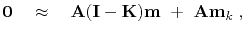
A second way to find missing data is with the set of goals:
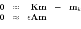 |
(44) |
and take the limit as the scalar
 .
At that limit, we should have the same result
as equation (43).
.
At that limit, we should have the same result
as equation (43).
There is an important philosophical difference between
the first method and the second.
The first method strictly honors the known data.
The second method acknowledges that when data misfits
the regularization theory, it might be the fault of the data,
so the data need not be strictly honored.
Just what balance is proper falls to the numerical choice of  ,
a nontrivial topic.
,
a nontrivial topic.
A third way to find missing data is to precondition
equation (44),
namely, try the substitution
 .
.
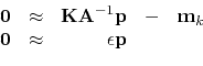 |
(45) |
There is no simple way of knowing beforehand
what is the best value of
.
Practitioners like to see solutions for various values of
.
Of course, that can cost a lot of computational effort.
Practical exploratory data analysis is more pragmatic.
Without a simple clear theoretical basis,
analysts generally begin from  and abandon the fitting goal
 .
Implicitly, they take
.
Implicitly, they take
 .
Then, they examine the solution as a function of iteration,
imagining that the solution at larger iterations
corresponds to smaller
.
There is an eigenvector analysis
indicating some kind of basis for this approach,
but I believe there is no firm guidance.
.
Then, they examine the solution as a function of iteration,
imagining that the solution at larger iterations
corresponds to smaller
.
There is an eigenvector analysis
indicating some kind of basis for this approach,
but I believe there is no firm guidance.
Subsections
Next: SeaBeam
Up: Preconditioning
Previous: INVERSE LINEAR INTERPOLATION
2015-05-07