 |
 |
 |
 | Simulating propagation of separated wave modes in general anisotropic media, Part I: qP-wave propagators |  |
![[pdf]](icons/pdf.png) |
Next: Bibliography
Up: Cheng & Kang: Propagation
Previous: Conclusions
The research leading to this paper was supported by the National Natural Science Foundation of China (No.41074083)
and the Fundamental Research Funds for the Central Universities (No.1350219123).
We would like to thank Sergey Fomel, Paul Fowler, Yu Zhang, Tengfei Wang and Chenlong Wang
for helpful discussions in the later period of this study.
Constructive comments by Joe Dellinger, Faqi Liu, Mirko van der Baan, Reynam Pestana, and an anonymous reviewer
are much appreciated. We thank SEG, HESS Corporation and BP for making the 2D VTI and TTI synthetic data sets available,
and the authors of Madagascar for providing this
software platform for reproducible computational experiments.
Appendix
A
Pseudo-pure-mode qP-wave equation for vertical TI and orthorhombic media
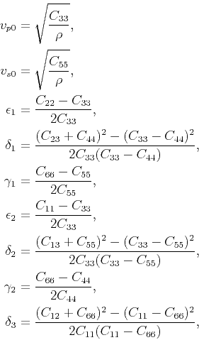
For vertical TI and orthorhombic media, the stiffness tensors have the same null components and can
be represented in a two-index notation (Musgrave, 1970) often called the “Voigt notation” as
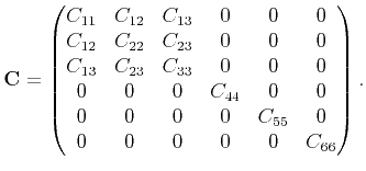 |
(34) |
For vertical orthorhombic tensor, the nine coefficients are indepedent, but the VTI tensor has only
five independent coefficients with
 ,
,
 ,
,
 and
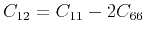
and
 .
The stability condition requires these parameters to satisfy the corresponding constraints (Helbig, 1994; Tsvankin, 2001).
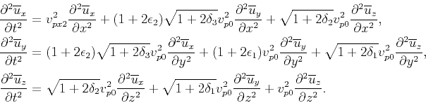
According to equations 3 and 4, the full elastic wave equation without the source terms is expressed as:
.
The stability condition requires these parameters to satisfy the corresponding constraints (Helbig, 1994; Tsvankin, 2001).
According to equations 3 and 4, the full elastic wave equation without the source terms is expressed as:
 |
(35) |
Thus the corresponding Christoffel matrix in wavenumber domain satisfies
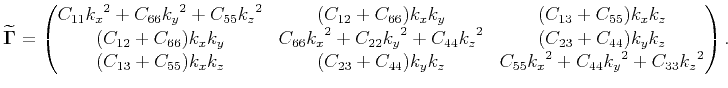 |
(36) |
According to equation 10, the Christoffel matrix after the similarity transformation is given as,
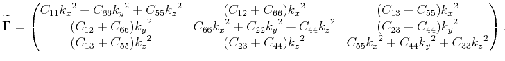 |
(37) |
Finally, we obtain the pseudo-pure-mode qP-wave equation (i.e., equation 18)
by inserting equation A-4 into equation 12 and applying an
inverse Fourier transform.
Appendix
B
Pseudo-pure-mode qP-wave equation in orthorhombic media
One of the most common reasons for orthorhombic anisotropy in sedimentary basins is a combination of parallel
vertical fractures and vertically transverse isotropy in the background medium (Schoenberg and Helbig, 1997; Wild and Crampin, 1991).
Vertically orthorhombic models have three mutually
orthogonal planes of mirror symmetry that coincide with the coordinate planes
![$ [x_{1},x_{2}]$](img126.png) ,
,
![$ [x_{1},x_{3}]$](img127.png) and
and
![$ [x_{2},x_{3}]$](img128.png) . Here we assume
. Here we assume  axis is the x-axis (and used as the symmetry axis),
 the y-axis, and
  the z-axis.
Using the Thomsen-style notation for orthorhombic media (Tsvankin, 1997):
the z-axis.
Using the Thomsen-style notation for orthorhombic media (Tsvankin, 1997):
 |
(38) |
and
 |
(39) |
the pseudo-pure-mode qP-wave equation (equation 18) is rewritten as,
 |
(40) |
where  represents the vertical velocity of qP-wave,
  represents the vertical velocity of qS-waves polarized
in the
direction,
represents the vertical velocity of qS-waves polarized
in the
direction,
 ,
,
 and
and
 represent the VTI parameters
  ,
,  and
and  in the
 ![$ [y,z]$](img139.png) plane,
plane,
 ,
,
 and
and
 represent the VTI parameters
,
and
in the
represent the VTI parameters
,
and
in the ![$ [x,z]$](img143.png) plane,
plane,
 represents the VTI parameter
in the
represents the VTI parameter
in the ![$ [x,y]$](img145.png) plane.
plane.  and
and  are the
horizontal velocities of qP-wave in the
symmetry planes normal to the x- and y-axis, respectively.
are the
horizontal velocities of qP-wave in the
symmetry planes normal to the x- and y-axis, respectively.
 ,
,  and
and  are the interval NMO velocities
in the three symmetry planes, and
are the interval NMO velocities
in the three symmetry planes, and
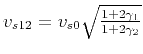 .
.
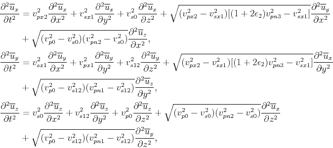
Setting  , we further obtain the pseudo-acoustic coupled system in a vertically orthorhombic media,
 |
(41) |
Note that this equation does not contain any of the parameters
and
that describe
the shear-wave velocities in the directions of the x- and y-axis, respectively.
Evidently, kinematic signatures of qP-waves in pseudo-acoustic
orthorhombic media depend on just five anisotropic coefficients (
,
,
,
and
) and the vertical velocity
.
In the presence of dipping fracture, we need to extend the vertically orthorhombic
symmetry to a more complex form, i.e. orthorhombic media with tilted symmetry planes.
Similar to TTI media, we locally rotate the coordinate system to make use of the simple form of the pseudo-pure-mode wave equations
in vertically orthorhombic media. Since the physical properties are not symmetric in the local
![$ [x_{1};x_{2}]$](img153.png) plane, we need three angles
to describe the rotation (Zhang and Zhang, 2011). Two angles,
plane, we need three angles
to describe the rotation (Zhang and Zhang, 2011). Two angles,  and
and  , are used to define the vertical axis at each
spatial point as we did for the symmetry axis in TTI model. The third angle
, are used to define the vertical axis at each
spatial point as we did for the symmetry axis in TTI model. The third angle  is introduced to rotate the stiffness tensor
on the local plane and to represent the orientation of the fracture system in a VTI background or the orientation of the first
fracture system of two orthogonal ones in an isotropic background.
is introduced to rotate the stiffness tensor
on the local plane and to represent the orientation of the fracture system in a VTI background or the orientation of the first
fracture system of two orthogonal ones in an isotropic background.
The second-order differential operators in the rotated coordinate system are expressed in
the same forms as in equation 28, but the rotation matrix is now given by,
 |
(42) |
where
 |
(43) |
Substituting the second-order differential operators into the rotated coordinate system for
those in the pseudo-pure-mode qP-wave equation
of vertically orthorhombic media yields the pseudo-pure-mode qP-wave equation of
tilted orthorhombic media in the global Cartesian coordinates.
Appendix
C
Deviation between phase normal and polarization direction of qP-waves in VTI media
For VTI media, Dellinger (1991) presents an expression of the deviation angle  between the phase normal
(with phase angle
between the phase normal
(with phase angle  ) and the polarization direction of qP-waves, namely
![$\displaystyle \sin^2(\zeta)=\frac{1}{2}+\frac{[(2s-1)t_{1}-t_{2}]\sqrt{t_{1}^2-t_{2}\chi}}{2(t_{2}\chi-{t_{1}}^2)},$](img158.png) |
(44) |
where
 |
(45) |
Equation C-1 indicates that the deviation angle has a complicated nonlinear relation with anisotropic parameters
and the phase angle. The relationship is rather lengthy and does not easily reveal the features caused by anisotropy.
Hence we use an alternative expression under a weak anisotropy assumption (Rommel, 1994; Tsvankin, 2001),
![$\displaystyle \zeta=\frac{[\delta+2(\epsilon-\delta)\sin^2{\psi}]\sin{2\psi}}{2(1-\frac{v_{s0}^2}{v_{p0}^2})}$](img160.png) |
(46) |
It appears that the deviation angle is mainly affected by the difference between
and
,
the magnitude of
(when
 stays the same) and the ratio of vertical velocities of
qP- and qS-wave, as well as the phase angle.
stays the same) and the ratio of vertical velocities of
qP- and qS-wave, as well as the phase angle.
|
|
|
|
| Simulating propagation of separated wave modes in general anisotropic media, Part I: qP-wave propagators | |
|
Next: Bibliography
Up: Cheng & Kang: Propagation
Previous: Conclusions
2014-06-24