 |
 |
 |
 | Simulating propagation of separated wave modes in general anisotropic media, Part I: qP-wave propagators |  |
![[pdf]](icons/pdf.png) |
Next: Pseudo-pure-mode qP-wave equation
Up: PSEUDO-PURE-MODE COUPLED SYSTEM FOR
Previous: PSEUDO-PURE-MODE COUPLED SYSTEM FOR
Vector and component notations are used alternatively throughout the paper. The wave equation in general
heterogeneous anisotropic media can be expressed as (Carcione, 2001),
![$\displaystyle \rho\frac{\partial^2\mathbf{u}}{\partial t^2} = [{\bigtriangledown}{\mathbf{C}{\bigtriangledown}^{T}}]\mathbf{u} + \mathbf{f},$](img3.png) |
(1) |
where
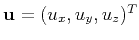 is the particle displacement vector,
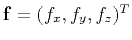 represents
the force term,
represents
the force term,  is the density,
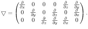
 is the matrix representing the stiffness tensor in a
two-index notation called the “Voigt recipe”, and the symmetric gradient operator has
the following matrix representation:
is the matrix representing the stiffness tensor in a
two-index notation called the “Voigt recipe”, and the symmetric gradient operator has
the following matrix representation:
 |
(2) |
Assuming that the material properties vary sufficiently slowly so that spatial derivatives of the stiffnesses
can be ignored, equation 1 can be simplified as
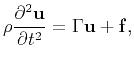 |
(3) |
where  is the
  symmetric Christoffel differential-operator matrix, of which the elements
are given for locally smooth media as follows (Auld, 1973),
symmetric Christoffel differential-operator matrix, of which the elements
are given for locally smooth media as follows (Auld, 1973),
 |
(4) |
For the most important types of seismic anisotropy such as transverse isotropy and orthorhombic anisotropy,
some terms in equation 4 vanish
because the corresponding stiffness coefficients become zeros.
Neglecting the source term, a plane-wave analysis of the elastic anisotropic wave equation yields the
Christoffel equation,
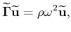 |
(5) |
or
 |
(6) |
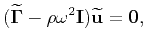
where  is the frequency,
 is the wavefield in Fourier domain,
 is the symmetric Christoffel matrix,
 is a
identity matrix.
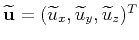
To support the sign notation in equations 5 and 6,
we remove the imaginary unit
is a
identity matrix.
To support the sign notation in equations 5 and 6,
we remove the imaginary unit  of the wavenumber-domain counterpart of the gradient operator
 and thus express matrix
 as:
as:
 |
(7) |
Setting the determinant of
 in equation 6 to zero gives the
characteristic equation, and expanding that determinant gives the (angular) dispersion relation. For a given
spatial direction specified by a wave vector
in equation 6 to zero gives the
characteristic equation, and expanding that determinant gives the (angular) dispersion relation. For a given
spatial direction specified by a wave vector
 , the characteristic equation
poses a standard
eigenvalue problem. The three eigenvalues correspond to the phase velocities of
the qP-wave and two qS waves. Inserting one of the eigenvalues back into the Christoffel equation gives
ratios of the components of
, the characteristic equation
poses a standard
eigenvalue problem. The three eigenvalues correspond to the phase velocities of
the qP-wave and two qS waves. Inserting one of the eigenvalues back into the Christoffel equation gives
ratios of the components of
 , from which the polarization or displacement direction
can be determined for the given wave mode. In general, these directions are neither parallel nor
perpendicular to the wave vector, and depend on the local material parameters for the anisotropic
medium. For a given wave vector or slowness direction, the polarization vectors of the three wave modes are
always mutually orthogonal.
, from which the polarization or displacement direction
can be determined for the given wave mode. In general, these directions are neither parallel nor
perpendicular to the wave vector, and depend on the local material parameters for the anisotropic
medium. For a given wave vector or slowness direction, the polarization vectors of the three wave modes are
always mutually orthogonal.
Applying an inverse Fourier transform to the dispersion relation yields a high-order PDE in time and space
and contains mixed space and time derivatives. Setting the shear velocity along the axis of symmetry to zero
while using Thomsen's parameter notation yields the pseudo-acoustic dispersion relation and wave equation
in VTI media (Alkhalifah, 2000). Most published methods instead
have used coupled PDEs (derived from the pseudo-acoustic dispersion relation) that are only second-order in time and
eliminate the mixed space-time derivatives, e.g., Zhou et al. (2006b). Many kinematically equivalent
coupled second-order systems can be generated from the dispersion relation
by similarity transformations (Fowler et al., 2010). In the next section, we present a particular similarity
transformation to the Christoffel equation in order to derive a minimal second-order coupled system,
which is helpful for simulating propagation of separated qP-waves in anisotropic media.
|
|
|
|
| Simulating propagation of separated wave modes in general anisotropic media, Part I: qP-wave propagators | |
|
Next: Pseudo-pure-mode qP-wave equation
Up: PSEUDO-PURE-MODE COUPLED SYSTEM FOR
Previous: PSEUDO-PURE-MODE COUPLED SYSTEM FOR
2014-06-24