Discussion

We first emphasize that one of the main advantages of time-domain processing is efficiency. Despite its well-known limitations in complex geologic environments (e.g., subsalt), it remains an attractive choice in some other important areas such as unconventional reservoirs, where the geology is largely layered (e.g, SEAM II model in Figure 17) and an expensive treatment of depth-imaging may not be necessary (Fomel, 2014). Our time-warping approach presented here further improves the current automatic time-domain processing workflow by proposing the use of highly accurate 3D traveltime approximations (equation 4) and adding a probabilistic component for a better analysis of the inversion results. We show that these additions can easily be implemented, while maintaining the original goal of efficiency and automation. We note, however, that the degree of efficiency of our time-warping approach primarily depends on the number of sampled models, which must be tailored to any specific problem on a case-by-case basis.

In addition, even though we propose a workflow with two inversion runs to help obtain better prior distributions for $W_i$ by taking advantage of one of the characteristics of our problem (i.e., $W_i$ can be estimated with only small-offset data), our resulting posterior probability distributions of $A_i$ are still estimated relative to the choice of uniform priori probability distributions. Therefore, it remains possible to improve the proposed approach if a better knowledge on the prior distributions $\rho(\mathbf{m})$ is available. For example, one may choose to use, instead of a uniform prior, a Gaussian distribution over some known mean value and standard deviation. Such information may be obtained on the basis of a previous velocity model in the region or any nearby well measurement. A better characterization of the prior probability distributions will surely enhance the efficiency of Monte Carlo sampling for solutions to the moveout inversion problem.

We note that in practice, it is sensible to consider a large range for uniform prior distributions of different parameters. However, this may not be the best choice in view of computational efficiency. We emphasize that this decision has to be made on a case-by-case basis and one may choose to follow our method by utilizing information such as relationships between GMA parameters and $\eta$ in equation 13, as well as, results from forward computational experiments with 3D GMA in various media (Sripanich et al., 2017) to help coming up with a rough numeric range for each parameter.

Moreover, one could be tempted to use a different inversion sequence (e.g., estimate $W_i$, $A_i$, and $S_{\%}$ before $B_i$ and $C_i$) with more runs to better constrain the results or to use a different parameterization as that in equation 4 to reduce the trade-offs between parameters. However, we would like to emphasize that $A_i$, $B_i$ and $C_i$ are inherently connected. 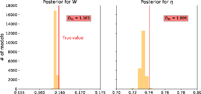This follows from the fact that to maintain the accuracy of moveout traveltime approximations, the quartic ($x^4$) term needs to have both the numerator (related to $A_i$) and the denominator (related to $B_i$ and $C_i$). Without a proper denominator, the series would lead to inferior accuracy (higher error) at large offsets (Tsvankin, 2012; Sripanich et al., 2017). Therefore, it is unclear how we can separately invert for $A_i$, $B_i$ and $C_i$ in different runs without introducing any potential bias to the results. One way to approximately handle this complexity is to assume a relationship among $A_i$, $B_i$, and $C_i$ such as that in equation 13, which effectively reduces the number of inverted parameters at the expense of the moveout approximation accuracy. The result from this experiment with our 2D inverse moveout example (Figure 3) is shown in Figure 27, where we can observe that the maximum likelihood points of estimated $W$ and $\eta$ lie close to the true values. Nonetheless, the 3D counterpart of equation 13 is not yet established for complex 3D layered orthorhombic media with azimuthally rotated principal axes such as the SEAM II model.

thist2D-eta
Figure 27. Estimated posterior probability distributions in the form of histograms from the proposed two-run inversion for the Dry Green River shale example with the $\eta$ constraint in equation 13. The maximum likelihood points are located close to the true values suggesting that moveout parameters from 2D gathers are well recoverable from the proposed approach.

In our inversion workflow, we propose to use the Metropolis-Hastings algorithm for its simplicity. There are more advanced guided random walk methods that can lead to better performance and several of them are reviewed by Sambridge and Mosegaard (2002). Other choices of likelihood functions $L(\mathbf{m})$ are also possible (Tarantola, 2005; Mosegaard and Tarantola, 1995). Nonetheless, it is expected that our observations on the characteristics of the resulting posterior probability distributions (i.e, multi-modal and diffuse) should remain valid.

With regard to the resulting posterior probability distributions, it is clear that there is non-uniqueness in the moveout inversion based on traveltime fitting and trade-offs between inverted parameters. Grechka and Tsvankin (1998b) show that the inverted nonhyperbolic moveout parameter— $\eta$ in their case— is highly sensitive to the errors in reflection traveltimes and the spreadlength of available data. This observation agrees with our posterior probability distributions that can be both multi-modal and diffuse, which suggest that there are many equivalently good sets of possible moveout parameters that satisfy the same level of accuracy in predicting reflection traveltimes. Moreover, the $B_i$ and $C_i$ in 3D GMA also remain undetermined and contribute to the non-uniqueness in the inverted models. Therefore, several factors contribute to the non-uniqueness of possible solutions and choosing which specific choice of representative model parameters to commit to is not straightforward. The results obtained from our approach could be used as starting models for more sophisticated tomographic or full-waveform inversion techniques for more accuracy and better convergence.

In the time-warping workflow, it is important to reiterate that we do not map local slopes to moveout parameters directly as that requires a prior assumption of the traveltime approximation form (Stovas and Fomel, 2016). Rather, we rely on measured slope fields and predictive painting to automatically trace CMP events and capture the moveout curves regardless of their shape. Consequently, conditioning of local slopes field is critical to the quality of the input traveltime data for the inversion. In light of this topic, it is possible to further improve the time-warping method by addressing potential problems that may arise from interfering dips (Schleicher et al., 2009) and predictive painting across discontinuties (Xue et al., 2018). Nonetheless, given that the information on reflection traveltimes can be obtained, our proposed Bayesian inversion will produce posterior distributions of estimated parameters that reflect the level of data uncertainty.

We stress that there are many possible choices of moveout approximations that can be used. Each of them can achieve a different level of approximation accuracy and involves a different set of moveout parameters. The 3D GMA is chosen here primarily due to its convenient applicability to complex 3D anisotropic models (e.g, layered orthorhombic with unaligned vertical symmetry planes in SEAM II) and its high accuracy in traveltime prediction, which technically allows us to accurately invert for moveout parameters and relate them to subsurface properties. This comes at a price of working with a large number of moveout parameters (seventeen). Other less accurate moveout approximations with fewer parameters can be used but a poorer performance in traveltime prediction may lead also to more uncertainty in the inverted moveout parameters. Nevertheless, an analysis has to be conducted on a case-by-case basis to draw meaningful conclusions regarding the trade-offs between the accuracy of traveltime approximation and the number of resolvable moveout parameters. Therefore, in general, it appears to be practicable to perform moveout inversion in a hierarchical manner starting from 3D GMA, which is applicable to a complex 3D model before reducing the number of inverted parameters based on resolvability of parameters (e.g., with an analysis on the posterior probability distributions and $D_{KL}$) or different assumptions such as a simpler anisotropic model of subsurface medium.

The estimated moveout parameters ($W_i$ and $A_i$) are well-known to also be affected by lateral heterogeneity (Sripanich et al., 2019; Grechka and Tsvankin, 1999; Blias, 2009; Lynn and Claerbout, 1982). Only when the subsurface is laterally homogeneous (1D) can the moveout parameters directly be related to medium parameters. In our approach, we do not specify their expressions explicitly in terms of medium parameters and treat them as `effective' moveout parameters that are estimated based on the 3D GMA. Interval parameter estimation can subsequently be accomplished by layer-stripping given that the medium is assumed to be 1D (Sripanich and Fomel, 2016; Koren and Ravve, 2017).

Most importantly, regardless of which moveout approximation one uses, the time-warping workflow, nonetheless, remains the same. The final estimated models are expressed in the time ($t_0$) domain, which can be related to the depth model via time-to-depth conversion (Sripanich and Fomel, 2018; Cameron et al., 2007; Li and Fomel, 2015).

Finally, we note that alternative traveltime approximations such as various forms of common-reflection-surface (CRS) approximations exist, which consider traveltime variations in both offset and midpoint directions (e.g., Jäger et al., 2001). In general, CRS methods aim to achieve better stacked images and objective functions for global CRS parameter estimation are normally considered based on coherency measurements such as semblance (e.g., Garabito, 2018; Barros et al., 2015; Bloot et al., 2018). An alternative estimation of CRS parameters can also be done by mapping directly from local slopes and curvatures (Waldeland et al., 2018; Santos et al., 2011). In view of the proposed approach, inversion-based CRS parameter estimation methods can potentially benefit from a Bayesian formulation, which will lead to statistical posterior distributions of estimated parameters. Nonetheless, in this study, we restrict ourselves to the CMP domain and the corresponding problem of parameter estimation from reflection moveout only in the offset direction. We focus on investigating the problem of 3D anisotropic model building at the earliest stage of processing from reflection moveouts. As demonstrated in our examples, the proposed framework is relatively flexible and can be used to bring additional statistical information on inverted parameters at any selected locations (reflectors). We anticipate that this method could represent an auxiliary tool that can help assess the quality of inverted moveout parameters from other automatic estimation methods.