Spiral-sorted (snail) gather

Instead of looking at 3D CMP gathers, Burnett (2011) shows that the time-warping workflow can accommodate gathers with other choices of sorting scheme, which may provide greater flexibility. This is due to the fact that in the time-warping workflow, one utilizes non-physical flattening that is not restricted to any particular event shape. The algorithm merely functions based on aligning events between neighboring traces and will be able to produce meaningful results as long as the automatic picker (predictive painting) can follow the events from trace to trace.

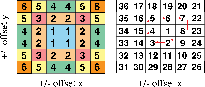
The first and most intuitive candidate is offset-sorted gather, where traces corresponding to the same CMP position is not binned but instead sorted and shown in 2D with increasing absolute offset. This leads directly to a practical advantage of requiring only 2D slope estimation as opposed to a 3D version. Additionally, neighboring CMP gathers can be offset-sorted and juxtaposed along the third axis for simultaneous processing with 3D slope estimator and additional regularization across CMP positions. Nonetheless, in this offset-sorting scheme, neighboring traces may be from completely random azimuths (Figure 22), which leads to a nonoptimal setup for capturing azimuthal variations of moveout curves.

spiral
Figure 22. Map-view setups for offset-sorted gather (left) and spiral-sorted gather (right). Different numbers indicate different traces that have to be sorted from the smallest to the largest. Azimuthal information in the former is arranged inconsistently because the absolute offsets are equal for all four traces and the order in which these four traces will be arranged is random. However, in the latter, the azimuthal information can be traced smoothly from small to large radial offsets, which enhances continuity and stability for the slope estimation process.

Alternatively, Burnett (2011) proposes that the choice of spiral sorting is particularly attractive because it holds a similar advantage of enabling the use of 2D slope estimator, yet captures azimuthal information. An illustration of a map-view spiral-sorted gather in comparison with offset-sorted gather is shown in Figure 22. We can see that spiral sorting the gather will allow the events to vary smoothly in both offset and azimuth, while maintaining a minimum physical proximity between neighboring traces.

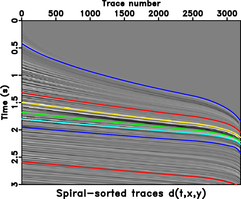
Using the same CMP gather of SEAM II data from the previous example, we spiral sort the gather instead of binning, which enables us to look at the total 3200 traces available at this particular CMP position. Subsequent 2D slope estimation, as opposed to 3D, is carried out and the automatically traced events are shown overlaying the spiral-sorted gather in Figure 23. We use the same prior distributions as in the previous case (Table 3) and the same general setup by recording the model every 500 samples with a total of 10,000 models. Similar histograms of estimated posterior distributions for the same two events are shown in Figures 24– 26. In this particular example of SEAM II data, apart from saving computational cost by allowing 2D slope estimation, spiral sorting the gather appears to slightly improve estimated posterior probability distributions in comparison with those from the previous section (Figures 19 and 20) — some of the maximum likelihood $A_i$ are closer to the 1D average values. Similar general observations and conclusions regarding the non-uniqueness of possible solutions can still be drawn.

pickongather
Figure 23. The spiral-sorted CMP gather of SEAM II model at $x$=4.375 km and $y$=2.881 km overlain by automatically picked events for non-physical flattening.

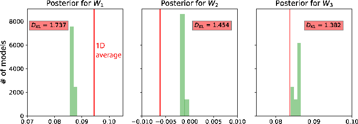
Whist0seamspi,Whist1seamspi
Figure 24. A comparison of estimated posterior probability distributions for $W_i$ in the form of histograms for events at (a) 1.315 $s$ and (b) 1.815 $s$ of the SEAM II model from the inversion with spiral-sorted gather. The solid vertical lines denote the 1D average values.

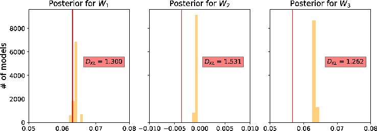
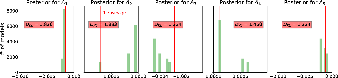
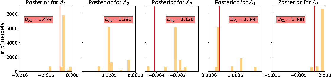
Ahist0seamspi,Ahist1seamspi
Figure 25. A comparison of estimated posterior probability distributions for $A_i$ in the form of histograms for events at (a) 1.315 $s$ and (b) 1.815 of the SEAM II model from the inversion with spiral-sorted gather. They are not as well-constrained as the inverted $W_1$ and $W_3$, which indicate large uncertainties. The solid vertical lines denote the 1D average values. However, some of the maximum likelihood $A_i$ are closer to the 1D average values than the results from regularly sorted gather (Figure 20).

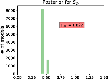
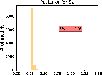
Shist0seamspi,Shist1seamspi
Figure 26. A comparison of estimated posterior probability distributions for $S_{\%}$ in the form of histograms for events at (a) 1.315 $s$ and (b) 1.815 of the SEAM II model from the inversion with spiral-sorted gather.