Dipping Isotropic Example

In the simple layered model, we assumed that the entire mis-tie is related to the vertical positioning of the reflector. However, as pointed out by Bakulin et al. (2010), solving the mis-tie equations along the axis of the well may result in biased estimates of velocities in the presence of dipping layers. To account for biased estimates of migration velocity updates due to dipping layers, we propose to migrate the data several times per iteration using perturbed velocity models. We use four percent increments to perturb the model. We then perform the seismic-well tie using each of the resulting seismic images and convert the mis-tie to a migration velocity update. We estimate the migration velocity update as the semblance weighted average of the velocity updates from each mis-tie.

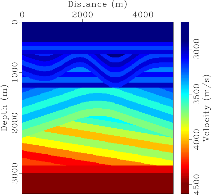
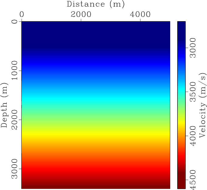
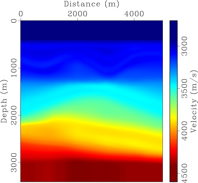
We model data using the true velocity model shown in Figure 6a, and the initial migration velocities are shown Figure 7a. We use a velocity profile from five `wells' located at 1000m, 2000m, 3000m, 4000m, and 5000m. With each iteration, we assume the velocity of the layer between 0m and 400m is known.

vel,vel2-2
Figure 6. (a) True velocity model. (b) One of the initial migration velocity model perturbations for the first iteration. The wells selected for well tie updates are located at 1000m, 2000m, 3000m, 4000m, and 5000m.

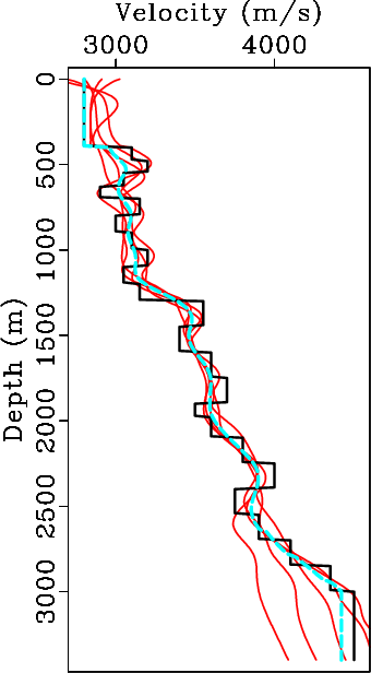
The seismic traces at locations 1000m, 2000m, 3000m, 4000m, and 5000m from each seismic image are stretched to time using the true well log velocity and the mis-ties is estimated using local similarity. Using Equation 7, we update the migration velocity at each well location. The results of migration velocity updates at well location 3000m for the five initial migration velocity models shown in Figure 7a are shown in Figure 7b. We spread the information along seismic structures using predictive painting weighted by radial basis functions to generate a new geologically consistent migration velocity model.

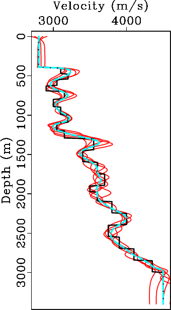
vels2,wellvel2-3,wellvel7-3
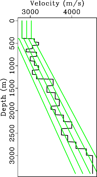
Figure 7. True velocity model at well location 3000m (black). (a) Starting migration velocity models with a linearly increasing velocity gradient (green). (b) Migration velocity updates from well tie updates based on the mistie between the synthetic seismogram modeled from the well log profile and the seismic image migrated from the five perturbed velocity models (red). Semblance weighted average of the five migration velocity updates (cyan), this result is used for interpolation of the next migration velocity model. (c) Results after six iterations of well tie updates.

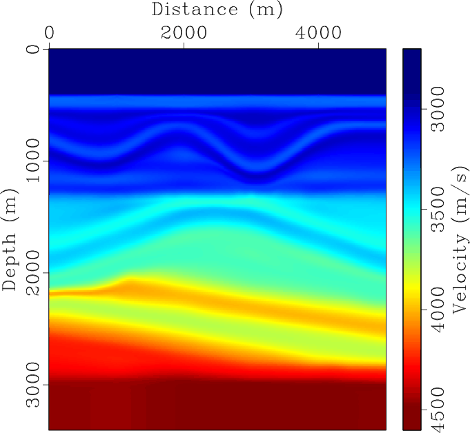
We iteratively update the migration velocity model by generating five perturbed migration velocity models at each iteration and estimating the semblance weighted average of the velocity updates from each mis-tie. Each iteration, we reduce the perturbation of the migration velocity models and the smoothing in local similarity. Results after six iterations of well tie updates at well location 3000m are shown in Figure 7c. We observe that the semblance weighted average of the velocity updates at this location fits well with the real well log velocity. The migration velocity model after six iterations is shown in Figure 8b and is reasonably consistent with the real velocity model in Figure 6a.

vel3,vel8
Figure 8. (a) Migration velocity model after one iteration and (b) six iterations of well tie updates and weighted interpolation of the updated velocity profile from the wells using predictive painting.

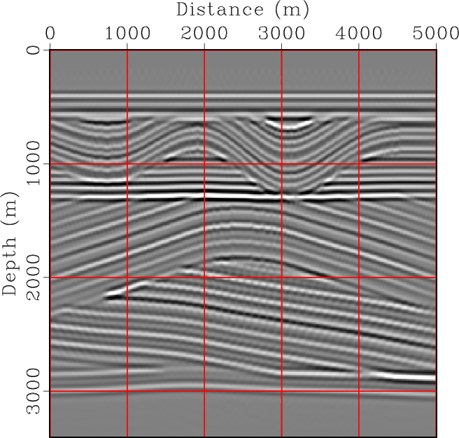
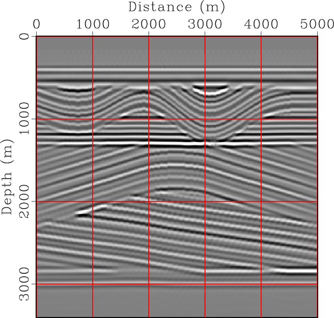
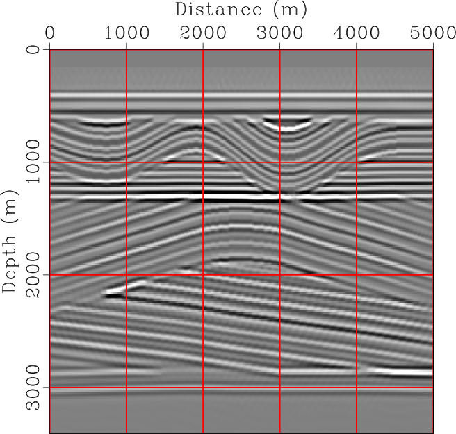
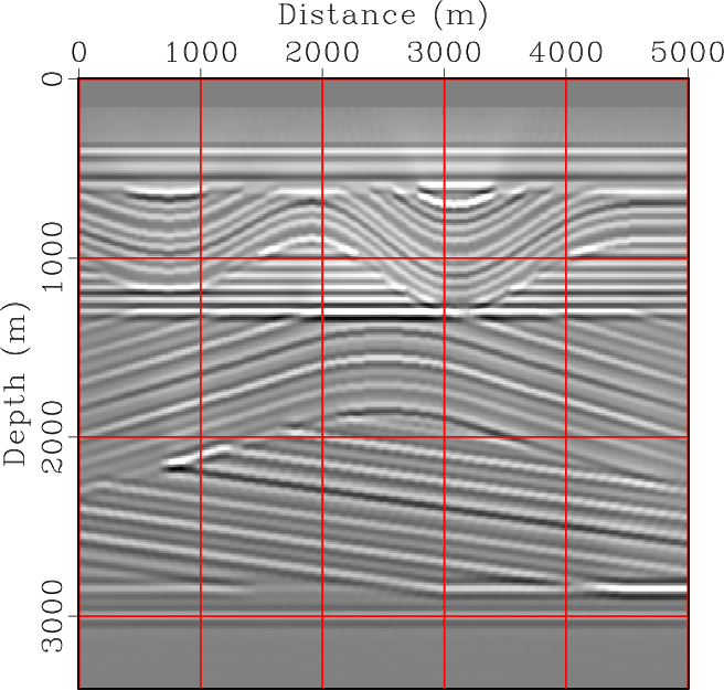
Figure 9c is the final depth migrated seismic image using the velocity model in Figure 8b. This result is compared against Figure 9d, the depth migrated seismic image using the real velocity model. Differences in the velocity models result is small differences in reflector positioning.

rtm2-2,rtm3-2,rtm8,rtm
Figure 9. (a) Initial RTM image using the migration velocity perturbation shown in Figure 6b. (b) RTM image using the migration velocity perturbation shown in Figure 8a. (c) Final RTM image using the migration velocity shown in Figure 8b after six iterations. (d) RTM image using the true migration velocity in Figure 6a.