|
|
|
|
Using well-seismic mistie to update the velocity model |
Next: Numerical Examples Up: Bader et al.: Update Previous: Introduction
|
|
|
|
Using well-seismic mistie to update the velocity model |
Seismic-well ties involve matching waveforms from a modeled synthetic seismogram with a nearby seismic trace (White and Simm, 2003). When comparing two datasets, our purpose is to estimate the warping function,  , required to align the synthetic seismogram,
  , with the seismic trace,
  ,
,
We can represent the warping function with time shifts,  , as follows:
 denotes the original independent axis and is the shifts required to match the datasets as defined in Equation 1. The LSIM method begins with the observation that the correlation coefficient only provides one number to describe the datasets in a defined window; however, we are interested in understanding the local changes in the datasets' similarity. Therefore, the LSIM method computes local similarity, which is a continuous function of time. The square of the correlation coefficient can be split into a product of two factors and posed as a regularized inversion where regularization operator is defined using shaping regularization and designed to enforce smoothness (Fomel, 2007a,b). From the similarity scan, we automatically pick the series of shifts along the entire length of the reference dataset that optimally aligns the two datasets (Fomel and Jin, 2009; Bader et al., 2017).
The relationship between the shifts estimated using LSIM and an updated velocity log assuming a TDR can be defined as:
where is the initial TDR,
  is the minimum depth at which sonic information is available,
  is the initial, upscaled, P-wave velocity from sonic and
  is the depth increment.
From Equation 2, assuming an initial TDR, , we arrive at
after one iteration of LSIM. We estimate a updated TDR by interpolating our shifts from time to depth
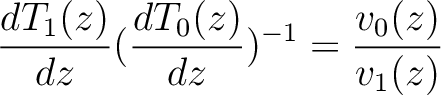
Using Equation 3, we relate the initial and updated velocity log to the initial and updated TDR,
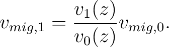
Muñoz and Hale (2015), Herrera et al. (2014), and Bader et al. (2018) use Equation 6 to estimate an updated velocity log. Alternatively, if we assume that the migration velocity model is consistent with velocities from logs, we update the migration velocity at the well location based on the proportion of the updated well log velocity to the initial well log velocity:
We use predictive painting (Fomel, 2010) to spread the updated migration velocity,
is the depth increment.
From Equation 2, assuming an initial TDR, , we arrive at
after one iteration of LSIM. We estimate a updated TDR by interpolating our shifts from time to depth
Using Equation 3, we relate the initial and updated velocity log to the initial and updated TDR,
Muñoz and Hale (2015), Herrera et al. (2014), and Bader et al. (2018) use Equation 6 to estimate an updated velocity log. Alternatively, if we assume that the migration velocity model is consistent with velocities from logs, we update the migration velocity at the well location based on the proportion of the updated well log velocity to the initial well log velocity:
We use predictive painting (Fomel, 2010) to spread the updated migration velocity,  , from the wells throughout the seismic volume. We weight the interpolation based on the distance between the reference well and any location in the seismic dataset using radial basis functions (Karimi et al., 2017).
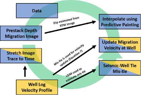
Using Equations 3–7, the migration velocity is iteratively updated using well tie updates. The seismic trace from the RTM depth image is stretched to time using the well log velocity profile and compared with the modeled synthetic seismogram from well logs. Figure 1 illustrates the workflow we use and is colored based on the data type used in each step.
|
|---|
|
capture
Figure 1. Workflow used in seismic-well tie velocity model updates. Blue indicates seismic data is used in the step. Yellow indicates well log data is used in the step. Black arrows indicate how the product of one step is used in a different step. |
|
|
|
|
|
|
Using well-seismic mistie to update the velocity model |