Three-layer model

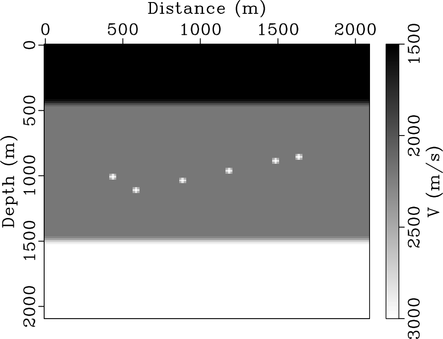
In the first example, we used a three-layer model with six assumed microseismic sources located within the middle layer (Figure 2a). The model is discretized on a 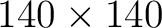$140 \times 140$ grid with $15\;m$ spacing in both vertical and horizontal directions. The model has sharp velocity contrasts, which generate multiple reflection events in both forward and backward propagation.

sov1,datatrace-clean,datatrace-noisy
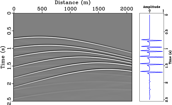
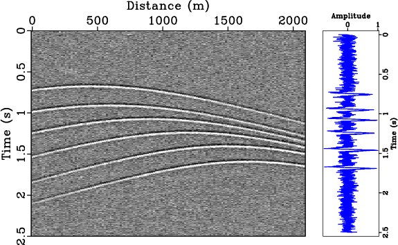
Figure 2. (a) Microseismic source locations overlaid on a three-layer velocity model. (b) Noise-Free microseismic data from three-layer model. (c) Noisy microseismic data from three-layer model. The traces displayed in the right panel correspond to $X=1050\;m$.

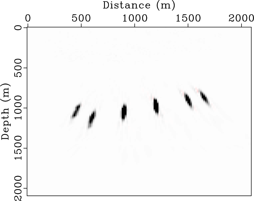
We first use noise-free data (Figure 2b) to test the sensitivity of the cross-correlation imaging condition to stratigraphic boundaries, which are common in unconventional reservoirs. We use data from only 10 surface stations starting from $X=75\;m$ and ending at $X=1965\;m$, with an interval of $210\;m$. After individually backward-propagating the receiver wavefields and applying the cross-correlation imaging condition (equation 1), we obtain a clean, high-resolution image which accurately locates all the correct hypocenters (Figure 3a).

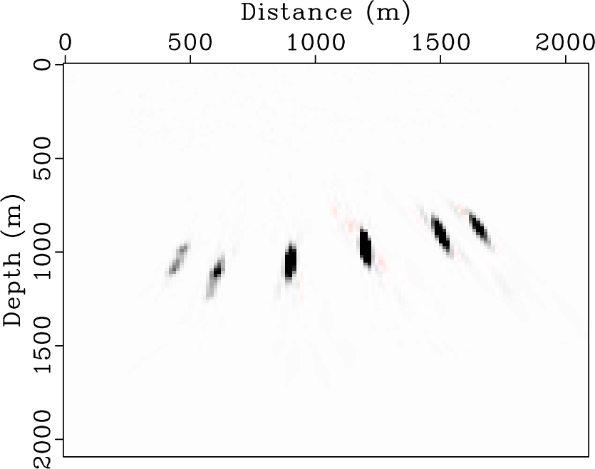
Next we introduce a strong random noise into the data (Figure 3b) to test the sensitivity of the method in such a setting. By keeping the number of receivers unchanged, the final image contains some false image points clustered around reflection boundaries. Additionally, although the image still contains all the true hypocenters, they are not well focused, i.e., some of the true hypocenters split across neighboring points.

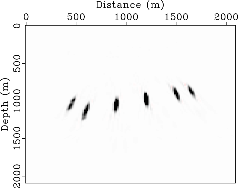
To remove the artifacts caused by a low SNR, we employ the hybrid imaging condition (equation 3) by including five receivers in one station. For example, the station at $X=75\;m$ now includes five receivers with an interval of $15\;m$. We still perform ten backward propagations, with each wavefield using data from five neighboring receivers. The image contains significantly less artifacts, with only one defocused point corresponding to the rightmost hypocenter (Figure 3c).

location0-clean,location0-noisy,location0-hyb
Figure 3. (a) Microseismic source locations imaged by the cross-correlation imaging condition using noise-free data. (b) Microseismic source locations imaged by the cross-correlation imaging condition using noisy data. (c) Microseismic source locations imaged by the hybrid imaging condition using noisy data.