|
|
|
|
Investigating the possibility of locating microseismic sources using distributed sensor networks |
Next: Numerical Examples Up: Sun et al.: Source Previous: Introduction
|
|
|
|
Investigating the possibility of locating microseismic sources using distributed sensor networks |
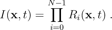
Motivated by the development of distributed sensor networks, we propose to adopt the imaging principle of prestack migration for locating microseismic hypocenters. We treat the wavefield back propagated from each individual receiver as an independent wavefield, and define microseismic hypocenters as the locations where all the wavefields coincide in both space and time. The imaging condition is formulated as a multiplication reduction of all the back propagated wavefields, calculated using data from each receiver:
A similar technique was developed by Nakata (2015, personal communication). Assuming the velocity model is accurate and data contains zero noise, the image should have non-zero values only if all the backward-propagated wavefields are non-zero at location
  and time
  , i.e., the starting of an earthquake. When noise is present in the data, extra non-zero values might appear in the image. However, as long as the noise has certain randomness, the amplitude of these false image points will be much weaker than those generated by coherent signal, and thresholding can effectively separate the non-zero values result from noise. The image
calculated by equation 1 therefore indicates the seismicity at time . The resolution of the image depends on the frequency content of the wavefields.
, i.e., the starting of an earthquake. When noise is present in the data, extra non-zero values might appear in the image. However, as long as the noise has certain randomness, the amplitude of these false image points will be much weaker than those generated by coherent signal, and thresholding can effectively separate the non-zero values result from noise. The image
calculated by equation 1 therefore indicates the seismicity at time . The resolution of the image depends on the frequency content of the wavefields.
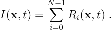
The conventional time-reversal imaging can be formulated in a similar fashion. Instead of performing multiplication, the image is produced by summing over all the receiver wavefields:
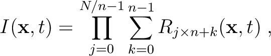
In practice, this is done by backward-propagating all the data at once and the summation is implicit. When applied to microseismic data from multiple sources, it is usually a challenging task to pick the hypocenters from the complicated wavefield, especially when the data has a low SNR.The cross-correlation imaging condition (equation 1) and time-reversal imaging condition (equation 2) represent two extremes. The image produced by equation 1 is high-resolution and easy to pick, since only non-zero values in the image correspond to hypocenters. However, it requires propagating the wavefields using data from each receiver separately, and thus is computationally intensive. Equation 2, on the other hand, requires essentially only one computation using the entire data set, but has less resolving power and is less suitable for distributed networks. A hybrid imaging condition would combine the merits of the two:
where is the local summation window length. Length should be selected such that neighboring receivers are backward-propagated together while far-apart receivers are cross-correlated. Equation 3 requires
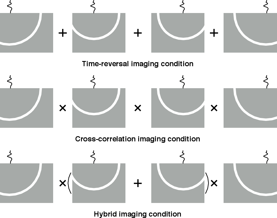
  computations of reverse-time modeling. In principle, both equation 1 and 3 need to perform cross-correlation using at least three wavefields to constrain one point in space. Schematically, the differences between the three imaging conditions is shown in Figure 1.
|
|---|
|
ic
Figure 1. Different imaging conditions for locating microseismic sources. A homogeneous medium and four receiver stations are assumed. A hybrid imaging condition calculates local summation before applying cross-correlation. In practice, the summation is performed implicitly by back propagating data from several neighboring receivers at once. |
|
|
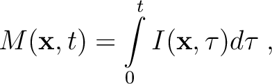
A movie of accumulated seismicity can be generated by performing an integration over time:
Movie is an evolving map of microseismicity in time that could be used to indicate rupture propagation. An image of all the sources corresponds the last instance of
.
is an evolving map of microseismicity in time that could be used to indicate rupture propagation. An image of all the sources corresponds the last instance of
.
|
|
|
|
Investigating the possibility of locating microseismic sources using distributed sensor networks |