Smoothing Filters and Edge Preservation

Smoothing is a filtering operation that aims to remove high-frequency noise from an input dataset. In general, there are two classes of smoothing filters: linear and non-linear (Hall, 2014). Linear filters such as stationary box and triangle filters smooth all input pixels in the same way, making them efficient. The general drawback of using linear smoothing filters is that they fail to preserve strong edges in the input dataset. Edge-preservation is essential in geophysical applications since edges contain important information such as faults, and channel boundaries (Bahorich and Farmer, 1995). Non-linear filters, on the other hand, can preserve or enhance strong edges, but they are costly relative to linear filters. Non-linear filters do not treat all input pixels in the same way; instead, they typically smooth an input pixel based on some statistical attribute of the pixels surrounding it. Examples of non-linear smoothing filters include a median filter, a bilateral filter, and an anisotropic diffusion filter (Perona and Malik, 1990; Tukey, 1970; Manduchi and Tomasi, 1998). We note that non-stationary triangle smoothing, a linear operator, can achieve both the low cost of linear filters and the edge-preserving ability of non-linear filters. The recursive implementation of non-stationary triangle smoothing costs exactly the same as stationary triangle smoothing. Furthermore, the non-stationary radius values can be tailored to the properties of the input dataset, for example, to adapt the strength of smoothing to the edges present.

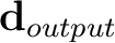
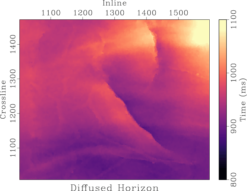
We compare the performance of non-stationary triangle smoothing against a select set of non-linear smoothing filters for a time horizon with added uniform noise of mean zero and range equal to 15 ms shown in Figure 1b. For reference, the original horizon without added noise is displayed in Figure 1a. We display the results of applying an $8\times 8$ median filter and an anisotropic diffusion filter to the noisy horizon in Figures 1c and 1d respectively. The result of applying a non-stationary triangle smoothing filter defined by the non-stationary radius values is displayed in Figure 2b. The non-stationary smoothing is applied in the horizontal direction only. To account for the smoothing required in the vertical direction, we apply vertical triangle smoothing using a small stationary radius equal to 2. The non-stationary radius is estimated using 5 iterations of the proposed method substituting the noisy horizon as $\mathbf{d}_{input}$ and the anisotropic diffusion-filtered horizon as $\mathbf{d}_{output}$. 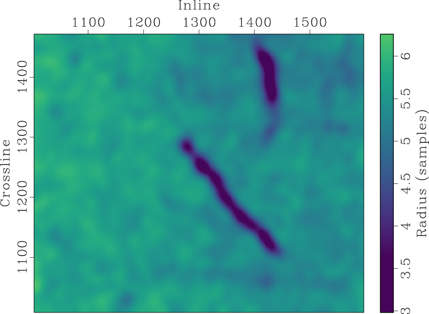The initial guess for the radius is a constant value equal to 4. The two strongest edges in the time horizon at inlines 1300 and 1400 correspond to small smoothing radius values, indicating that the estimated radius is adaptive to the edges present. The times required to compute the median-filtered horizon, the anisotropic diffusion-filtered horizon, and the non-stationary triangle-filtered horizon are 2.10 s, 1.62 s, and 0.02 s respectively. The iterative non-stationary radius estimation step takes 0.34 s. These comparisons are based on a MacBook Pro laptop with a 3.2 GHz M1 8-core processor. We plot time slices at crossline 1400 for the original time horizon, the noisy horizon, and the three filtered horizons in Figure 3. The horizon slices indicate that anisotropic diffusion does a better job at preserving edges in the original horizon compared to median filtering. The non-stationary triangle filter was designed to mimic the anisotropic diffusion filter, and we observe that the non-stationary triangle-filtered horizon slice does indeed mimic the characteristics of the anisotropic diffusion-filtered horizon slice.Thus, when taking efficiency into account, non-stationary smoothing can be the most practical edge-preserving filter especially for large multidimensional datasets.

filled,noisy,median,diffused
Figure 1. Time horizon example. (a) Original time horizon. (b) Horizon with added uniform noise of mean zero and range equal to 15 ms. (c) Noisy horizon smoothed with an $8\times 8$ median filter. (d) Noisy horizon smoothed with an anisotropic diffusion filter.

new-rect50,smooth-5
Figure 2. Time horizon example. (a) Non-stationary triangle smoothing radius. (f) Noisy horizon smoothed in the horizontal direction with a triangle filter defined by non-stationary radius values in (a), and in the vertical direction with a stationary radius equal to 2.

slice-test
Figure 3. Time horizon example. Time slices at crossline 1400 offset from each other by integer multiples of 200 ms for original time horizon (blue), noisy horizon (orange), median-filtered horizon (green), anisotropic diffusion-filtered horizon (red), and non-stationary triangle-filtered horizon (purple). Edges in the original time horizon indicated by dashed grey lines.