Marmousi Q model

vel,q
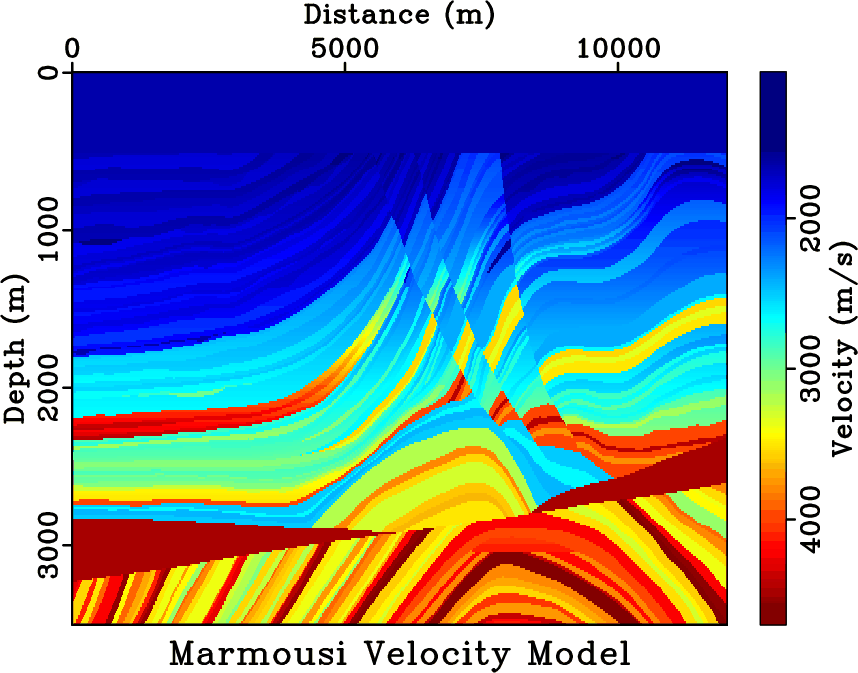
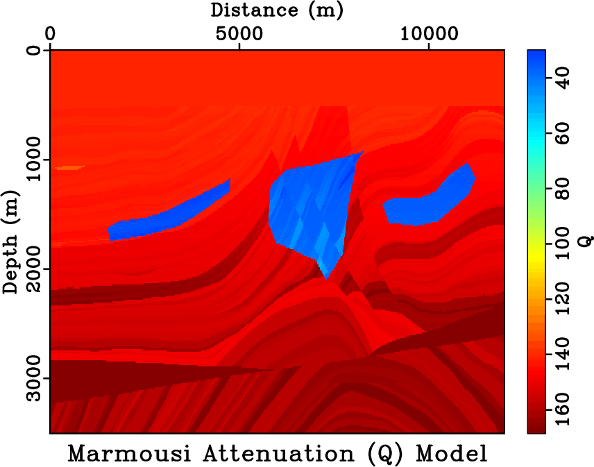
Figure 3. Marmousi velocity/attenuation ($Q$) model. (a) Marmousi velocity model; (b) Marmousi $Q$ model.

acudata,visdata,visdata-n
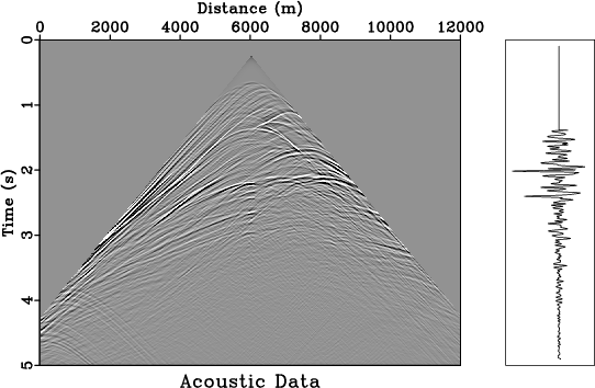
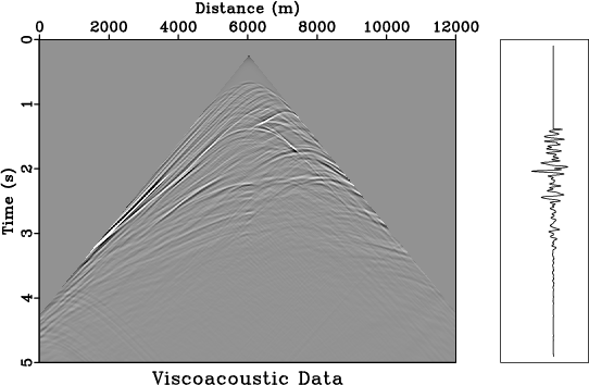
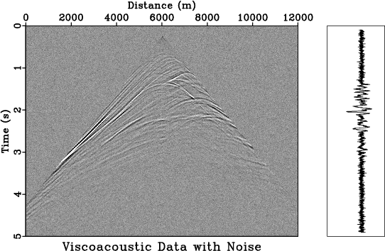
Figure 4. Common-shot gathers used for RTM and $Q$-RTM at $X=6025\;m$. A total length of $8\;s$ has been recorded, while only the first $5\;s$ is displayed. (a) Acoustic data; (b) viscoacoustic data. (c) viscoacoustic data with added random noise (SNR = $0.8$). The right panel shows a trace extracted from $X=4375\;m$.

acuimg,visimg,comimg
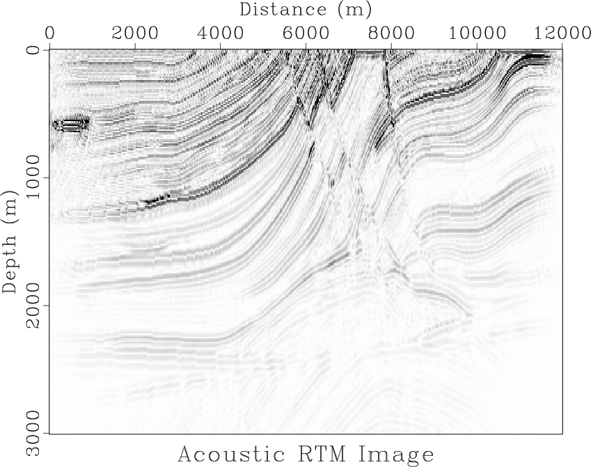
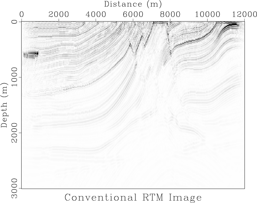
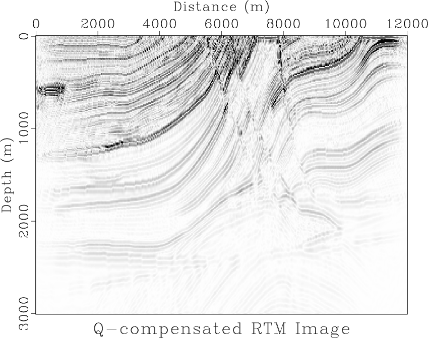
Figure 5. RTM images obtained using acoustic and visco-acoustic data. (a) Acoustic RTM image using acoustic data; (b) Acoustic RTM image using viscoacoustic data. (c) Q-RTM image using viscoacoustic data.

visacu,comacu,comacu-n
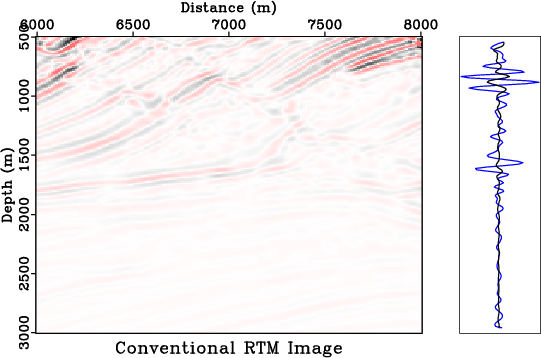
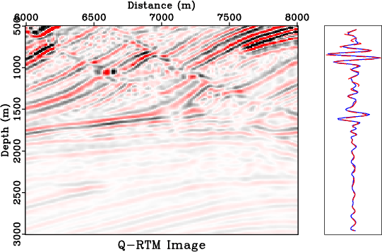
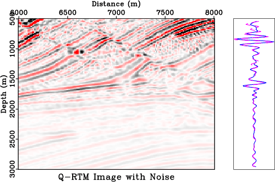
Figure 6. A portion of RTM images obtained using different approaches. (a) acoustic RTM image using viscoacoustic data; (b) $Q$-RTM image using viscoacoustic data; (c) $Q$-RTM image using viscoacoustic data with added noise. The right panel compares the trace at $X=6875\;m$ from the corresponding image with the reference image obtained by applying acoustic RTM on acoustic data. Blue solid line refers to the reference image; black solid line refers to the non-compensated image; red dashed line refers to the compensated image; pink dashed line refers to the compensated image using noisy data.

In the second example, we use a synthetic attenuation model to investigate the effect of $Q$ compensation in RTM. Figure 3a shows the Marmousi velocity model. We build a corresponding $Q$ model (Figure 3b) on the same grid. The model features three highly attenuative zones in the shallow parts of the model. This kind of an attenuation patter can be caused in reality by the presence of a gas accumulation. The model is discretized on a $241 \times 961$ grid with a spacing of $12.5\;m$ in both horizontal and vertical directions. A total of 64 shots with a horizontal spacing of $187.5\;m$ were used, starting from $25\;m$, and the source is a Ricker wavelet with a peak frequency of $20\;Hz$. Receivers have a spacing of $12.5\;m$, starting from $0\;m$ and ending at $12000\;m$. For simplicity of modeling, both sources and receivers are located at $-62.5\;m$ depth. The data have a temporal sampling of $2\;ms$, with a total length of $8\;s$. First, acoustic modeling is used to generate acoustic data (Figure 4a), and then viscoacoustic modeling is used to generate viscoacoustic data (Figure 4b), accounting for seismic attenuation during wave propagation. We first apply acoustic RTM on the (non-attenuated) acoustic data to generate a reference image (Figure 5a). The image generated by non-compensated RTM using viscoacoustic data (Figure 5b) suffers from a lack of illumination within and below the attenuative region. Using the proposed $Q$-RTM according to equations 17 and 18 (Figure 5c), the amplitude of the parallel normal faults and anticline structures has been recovered to a large extent, and image resolution inside and below gas has been greatly enhanced. The Tukey filter is applied with a cutoff frequency of $100\;Hz$ with a taper ratio of $0.4$. We extract the trace at $X=6875\;m$ and $Z$ between $500\;m$ and $3000\;m$ from the three images, and use the acoustic RTM image from migrating acoustic data as a reference (shown in Figures 6a and 6b). The comparison shows that the conventional RTM applied to viscoacoustic data suffers from the effects of phase rotation and amplitude attenuation, especially in the deeper part of the image, while the $Q$-compensated image highly resembles the non-attenuated acoustic image in both amplitude and phase. To test the sensitivity of the proposed method to noise in the data, we add Gaussian random noise to the viscoacoustic data with a signal-to-noise ratio (SNR) of $0.9$ (Figure 4c). Applying $Q$-RTM to the noisy data leads to a slightly noisier image (Figure 6c). However, migration remains stable and all the reflectors remain well-imaged.