|
|
|
|
Viscoacoustic modeling and imaging using low-rank approximation |
Next: Marmousi Q model Up: Numerical Examples Previous: Numerical Examples
|
|
|
|
Viscoacoustic modeling and imaging using low-rank approximation |
The purpose of our first example is to investigate the accuracy of the solution of the constant-![]() wave equation using the proposed low-rank scheme, in the presence of a sharp contrast in both velocity and
wave equation using the proposed low-rank scheme, in the presence of a sharp contrast in both velocity and ![]() . We use an isotropic two-layer model with
. We use an isotropic two-layer model with
![]() in the top layer and
in the top layer and
![]() in the bottom layer. The model is discretized on a
in the bottom layer. The model is discretized on a
![]() grid, with a spatial sampling of
grid, with a spatial sampling of ![]() along both
along both ![]() and
and ![]() directions. An explosive source with a peak frequency of
directions. An explosive source with a peak frequency of ![]() is located at the center. The reference frequency is
is located at the center. The reference frequency is
![]() . Wavefield snapshots are taken at
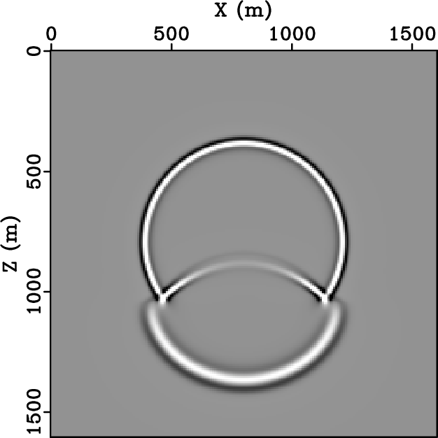
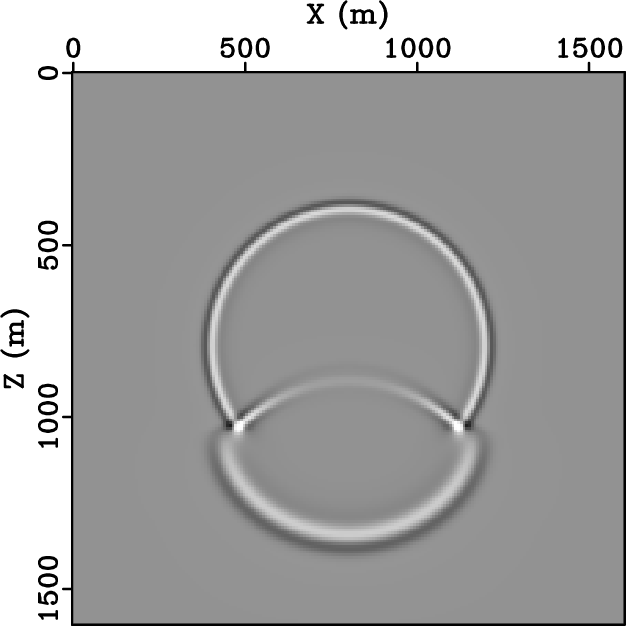
. Wavefield snapshots are taken at ![]() . Figure 1a shows the acoustic case, in which the model has the velocity discontinuity but no attenuation (
. Figure 1a shows the acoustic case, in which the model has the velocity discontinuity but no attenuation (![]() ). For comparison, Figure 1b demonstrates the effect of homogeneous attenuation where
). For comparison, Figure 1b demonstrates the effect of homogeneous attenuation where ![]() . Both velocity dispersion and amplitude loss can be observed. In Figure 1c, we set
. Both velocity dispersion and amplitude loss can be observed. In Figure 1c, we set ![]() in the top layer and
in the top layer and ![]() in the bottom layer. The transmitted arrival exhibits less attenuation compared with that in Figure 1b. In Figure 1d, both velocity and
in the bottom layer. The transmitted arrival exhibits less attenuation compared with that in Figure 1b. In Figure 1d, both velocity and ![]() remain the same as those in Figure 1c; however, the fractional power of Laplacians,
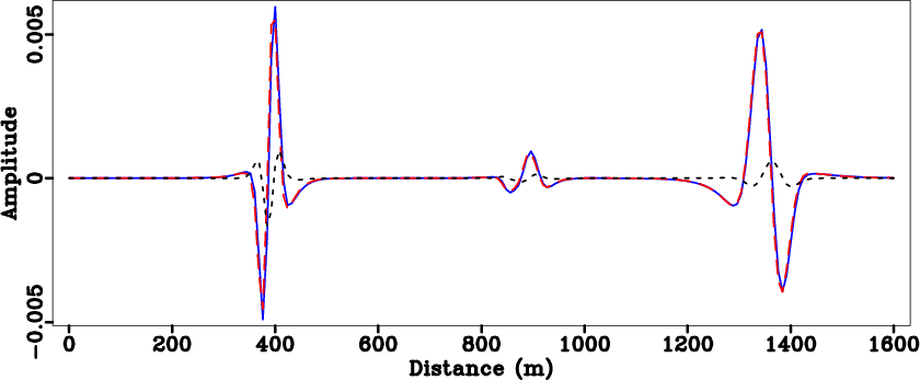
remain the same as those in Figure 1c; however, the fractional power of Laplacians, ![]() , is taken to be the averaged value, which corresponds to the original implementation by Zhu and Harris (2014). To compare the results modeled by the two strategies, a middle trace at
, is taken to be the averaged value, which corresponds to the original implementation by Zhu and Harris (2014). To compare the results modeled by the two strategies, a middle trace at ![]() is extracted from both wavefield snapshots (Figures 1c and 1d). Figure 2 shows the two traces, along with their difference. Errors caused by using a constant
is extracted from both wavefield snapshots (Figures 1c and 1d). Figure 2 shows the two traces, along with their difference. Errors caused by using a constant ![]() instead of a spatially varying
instead of a spatially varying ![]() can be easily observed.
can be easily observed.


|
|---|
|
snap-0,snap-1,snap-3,snap-4
Figure 1. Viscoacoustic wave propagation in a two-layer model: (a) acoustic modeling with |
|
|
|
|---|
|
cross
Figure 2. Traces at |
|
|
|
|
|
|
Viscoacoustic modeling and imaging using low-rank approximation |