 |
 |
 |
 | Double sparsity dictionary for seismic noise attenuation |  |
![[pdf]](icons/pdf.png) |
Next: Seislet transform based DSD
Up: Theory
Previous: Learning DSD in data
In order to perform optimization in equations 4 and 5, we can employ the data-driven approach that was suggested previously by Cai et al. (2013). As an example, we only introduce the solver for equation 5.
The minimization can be solved by updating coefficients of vector
 and the learning-based dictionary
 alternately. We adopt the following algorithm for solving problem 5:
Input: Base dictionary
 , initial learning-based dictionary
 .
.
- Transform data from data domain to model domain according to
 |
(6) |
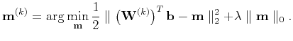
- for
 :
:
- Fix the learning-based dictionary
 , estimate the double-sparsity coefficients vector
 by
by
 |
(7) |
- Given the double-sparsity coefficients vector
, update the learning-based dictionary
 :
:
 |
(8) |
end for
After  iterations, the DSD coefficients are obtained and the observed data become sparsely represented by DSD.
It is known that minimization 7 has a unique solution
iterations, the DSD coefficients are obtained and the observed data become sparsely represented by DSD.
It is known that minimization 7 has a unique solution
 provided by applying a hard thresholding operator on the coefficient vector
 . The minimization 8 can be implemented by using a SVD-based optimization approach (Cai et al., 2013).
Assuming the size of the coefficients domain is
 , and
, and  , let a filter mapping
 be the block-wise Toeplitz matrix representing the convolution operator with a finitely supported 2D filter
 under the Newmann boundary condition. The learning based dictionary
 can be defined as
![$\displaystyle \mathbf{W} = \left[\mathbf{F}_{\mathbf{a}_1},\mathbf{F}_{\mathbf{a}_2},\cdots,\mathbf{F}_{\mathbf{a}_p} \right].$](img46.png) |
(9) |
Each
 is a 2D filter associated with a tight frame and the columns of
form a tight frame for
is a 2D filter associated with a tight frame and the columns of
form a tight frame for
 .
.  denotes the number of filters. The patch size discussed in the following examples corresponds to the size of each
.
denotes the number of filters. The patch size discussed in the following examples corresponds to the size of each
.
Liang et al. (2014) give an example of using spline wavelets for the initial
 and the finally learned dictionary
 . Following Liang et al. (2014), we also choose spline wavelets for the initial
.
. Following Liang et al. (2014), we also choose spline wavelets for the initial
.
|
|
|
|
| Double sparsity dictionary for seismic noise attenuation | |
|
Next: Seislet transform based DSD
Up: Theory
Previous: Learning DSD in data
2016-02-27