Discussion

It is worth emphasizing that even though we rely on the accuracy of traveltime predictions to verify the effectiveness of our proposed framework, it is not intended to be used in place of other numerical methods that can compute the traveltime derivatives more accurately such as the paraxial ray theory. 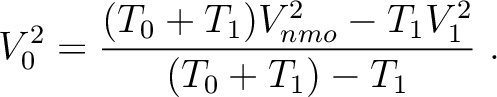The importance of our work lies in its contribution to the fundamental understanding on how effects from lateral heterogeneity can be characterized (derivatives of $F$ and $W$) and on how they can affect the parameters—normal-moveout velocity and time-migration velocity—we routinely use in time processing. The relationship between traveltime derivatives at different surfaces that leads to the recursion (equation 12) employed in this study is also closely related to that used in the development of important processing techniques such as Dix inversion. To elaborate on this final point further, we can take, for example, the relationship for a two-layered medium given by equation 43,

$$\frac{\partial^2 t}{\partial h^2} = \frac{\partial^2 t_1}{\partia... ...\middle/ \left(\frac{\partial^2 (t_0+t_1) }{ \partial x_1^2} \right) \right. ~.$$ (22)

For horizontal homogeneous isotropic sublayers, the pertaining traveltime derivatives can be expressed as

$$\left. \frac{\partial^2 t_1 }{\partial h^2} \right\rvert_{h=0} = \frac{1}{D_1/W_1} = \frac{1}{T_1V^2_1}~,$$ (23)

$$\left. \frac{\partial^2 t_1 }{ \partial x_1 \partial h} \right\rvert_{h=0} = -\frac{1}{D_1/W_1} = -\frac{1}{T_1V^2_1} ~,$$

$$\left. \frac{\partial^2 t_0 }{ \partial x_1^2} \right\rvert_{h=0} = \frac{1}{D_0/W_0} = \frac{1}{T_0V^2_0} ~,$$

$$\left. \frac{\partial^2 t_1 }{ \partial x_1^2} \right\rvert_{h=0} = \frac{1}{D_1/W_1} = \frac{1}{T_1V^2_1}~,$$

where $D_k$ is the thickness of the $k$-th layer and $V_k=1/W_k$ denotes its velocity. Substituting equation 23 into equation 22 gives

$$\left.\frac{\partial^2 t}{\partial h^2}\right\rvert_{h=0} = ~ \frac{1}{T_1V^2_1} - \left. \left(-\frac{1}{T_1V^2_1}\right)^2 \middle/ \left(\frac{1}{T_0V^2_0} + \frac{1}{T_1V^2_1} \right) \right.~,$$

$$= ~ \frac{1}{T_0V^2_0 + T_1V^2_1}~,$$ (24)

which leads to

$$V^2_{nmo} = ~\left[ (T_0+T_1) \left.\frac{\partial^2 t}{\partial h^2 }\right\rvert_{h=0} \right]^{-1}~,$$

$$= ~\frac{T_0V^2_0 + T_1V^2_1}{T_0+T_1}~.$$ (25)

Equation 25 serves as the basis for computing the effective NMO velocity, which is similar to the root-mean-square (RMS) velocity in this simple case. Dix-type inversion in this example follows directly from equation 25, where one seeks to estimate the velocity at the bottom layer $V_0$ from a measured $V_{nmo}$ at the surface according to

$$V^2_0 = \frac{(T_0+T_1)V^2_{nmo} - T_1 V^2_1}{(T_0+T_1) - T_1}~.$$ (26)

Alternative derivations for Dix-type inversion can be done in the phase domain, where the traveltime and offsets are expressed as functions of ray parameters (Sripanich and Fomel, 2016; Koren and Ravve, 2017; Tsvankin, 2012). Future investigations are required to establish a Dix-type inversion approach that honors the effects from lateral heterogeneity based on the result of this work.

Another possible extension of this work is to apply the proposed theory in the context of velocity anomaly removal similar to Blias (2009a), Takanashi and Tsvankin (2011), and Takanashi and Tsvankin (2012). In light of our result on the need of a recursive relationship (equation 12) to collect lateral heterogeneity effects from both curved interfaces and variable medium parameters, it remains to be investigated how the contribution from any individual layer with embedded velocity anomaly can be removed in an accurate and efficient manner.

The proposed method takes into account the effects from lateral heterogeneity by modifying the second-order traveltime derivative related to NMO velocity (reflection) or time-migration velocity (diffraction). Therefore, the limit on the validity of the hyperbolic traveltime assumption in both cases is still enforced. We further discuss the possibility of extending our framework to higher-order traveltime derivatives in Appendix D, where the conventional paraxial ray theory is no longer applicable. A possible 3D extension of the proposed framework is investigated in Appendix E, where we observe that an additional solve of a linear system of equations at each interface surface is needed to track the higher number of pertaining parameters in 3D. However, a direct solve of this system is generally not possible due to a smaller number of equations than unknowns. This problem was conveniently circumvented in the 2D case due to the smaller number of associated parameter (only one) and the use of a recursive relationship, which is no longer straightforward to formulate in the 3D case. Consequently, further investigations are required to extend the proposed framework to work with 3D datasets.

Our method takes into account the first-order effects from lateral heterogeneity in largely flat subsurface, which ensures that the normal-incidence ray and the image ray stays close to the reference vertical direction. Consequently, our approach does not substitute the dip-moveout process (DMO) for handling effects from dipping reflectors, which becomes prominent as the dip increases. The Gardner continuation (Fomel, 2014) serves as an alternative means to rid the moveout velocity on its dip dependency by transforming the prestack data into a special domain.

In our framework, we choose to consider the traveltime expression in the group domain, where it depends on the medium parameters and the spatial location in Cartesian coordinates. This choice allows for practical convenience when considering information at the zero offset and is appropriate for predominantly horizontally layered media with weak heterogeneity effects such as in land datasets associated with unconventional reservoirs. An alternative formulation can also be constructed in the phase domain, which can be advantageous when considering more complex media with arbitrarily dipping interfaces (Grechka et al., 2002; Grechka and Tsvankin, 2002).

Finally, we note that the results from this study, coupled with accurate moveout functional forms (Sripanich et al., 2017; Fomel and Stovas, 2010), may serve as the basis for possible future improvements of practical moveout inversion techniques that take into account the lateral heterogeneity effects. Subsequent applications of time-to-depth conversion methods that also honor lateral heterogeneity can potentially lead to an improved time-domain imaging workflow and a more accurate subsurface velocity model efficiently obtained from time processing (Cameron et al., 2007; Li and Fomel, 2015; Valente et al., 2017; Sripanich and Fomel, 2018). The latter is especially favorable as it may represent a good starting model for more sophisticated tomographic or full-waveform inversion techniques and lead to better convergence.