|
 |
 |
 | Nonhyperbolic reflection moveout of  -waves:
An overview and comparison of reasons -waves:
An overview and comparison of reasons |  |
![[pdf]](icons/pdf.png) |
Next: Vertically heterogeneous VTI model
Up: VERTICAL HETEROGENEITY
Previous: VERTICAL HETEROGENEITY
Nonhyperbolicity of reflection moveout in vertically heterogeneous
isotropic media has been extensively studied using the
Taylor series expansion in the powers of the offset
(Bolshykh, 1956; Taner and Koehler, 1969; Al-Chalabi, 1973). The most important property of
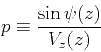
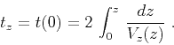
vertically heterogeneous media is that the ray parameter
does not change along
any given ray (Snell's law). This fact leads to the explicit parametric
relationships
where
 |
(21) |
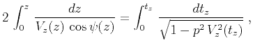
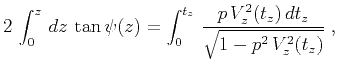
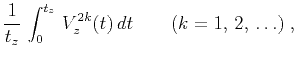
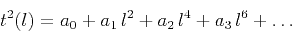
Straightforward differentiation of parametric equations (19)
and (20) yields the first four coefficients of the Taylor
series expansion
 |
(22) |
in the vicinity of the vertical zero-offset ray. Series
(22) contains only even powers of the offset  because
of the reciprocity principle: the pure-mode reflection traveltime is an even
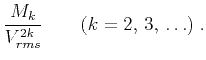
function of the offset. The Taylor series coefficients for the isotropic case
are defined as follows:
because
of the reciprocity principle: the pure-mode reflection traveltime is an even
function of the offset. The Taylor series coefficients for the isotropic case
are defined as follows:
where
 |
|
|
(27) |
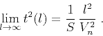
Equation (24) shows that, at small offsets, the reflection
moveout has a hyperbolic form with the normal-moveout velocity  equal to the root-mean-square velocity
  . At large offsets,
however, the hyperbolic approximation is no longer accurate. Studying
the Taylor series expansion (22), Malovichko (1978)
introduced a three-parameter approximation for the reflection
traveltime in vertically heterogeneous isotropic media.
His equation has the form of a
shifted hyperbola (Castle, 1988; de Bazelaire, 1988):
. At large offsets,
however, the hyperbolic approximation is no longer accurate. Studying
the Taylor series expansion (22), Malovichko (1978)
introduced a three-parameter approximation for the reflection
traveltime in vertically heterogeneous isotropic media.
His equation has the form of a
shifted hyperbola (Castle, 1988; de Bazelaire, 1988):
 |
(30) |
If we set the zero-offset traveltime  equal to the vertical
traveltime
equal to the vertical
traveltime  , the velocity equal to , and the parameter of heterogeneity
  equal to
  , equation
(30) guarantees the correct coefficients
, equation
(30) guarantees the correct coefficients  ,
,  , and
, and
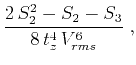
 in the Taylor series (22). Note that the parameter
is related to the variance
in the Taylor series (22). Note that the parameter
is related to the variance  of the squared velocity
distribution, as follows:
of the squared velocity
distribution, as follows:
 |
(31) |
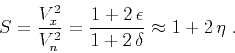
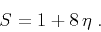
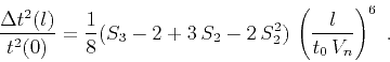
According to equation (31), this parameter is always greater
than unity (it equals 1 in homogeneous media). In many
practical cases, the value of lies between  and
and  . We can
roughly estimate the accuracy of approximation (30) at
large offsets by comparing the fourth term of its Taylor series with
the fourth term of the exact traveltime expansion (22).
According to this estimate, the error of Malovichko's approximation is
. We can
roughly estimate the accuracy of approximation (30) at
large offsets by comparing the fourth term of its Taylor series with
the fourth term of the exact traveltime expansion (22).
According to this estimate, the error of Malovichko's approximation is
 |
(32) |
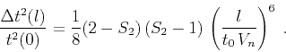
As follows from the definition of the parameters  [equations (29)] and the Cauchy-Schwartz inequality, the expression
(32) is always nonnegative.
This means that the shifted-hyperbola approximation
tends to overestimate traveltimes at large offsets. As the offset
approaches infinity, the limit of this approximation is
[equations (29)] and the Cauchy-Schwartz inequality, the expression
(32) is always nonnegative.
This means that the shifted-hyperbola approximation
tends to overestimate traveltimes at large offsets. As the offset
approaches infinity, the limit of this approximation is
 |
(33) |
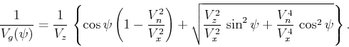
Equation (33) indicates that the effective horizontal
velocity for Malovichko's approximation (the slope of the shifted
hyperbola asymptote) differs from the normal-moveout velocity. One
can interpret this difference as evidence of some effective
depth-variant anisotropy. However, the anisotropy implied in
equation (30) differs from the true anisotropy in a
homogeneous transversely isotropic medium [see equation (1)].
To reveal this difference, let us substitute
the effective values
 ,
,
 ,
,
 , and
, and
 into equation (30). After eliminating the
variables
into equation (30). After eliminating the
variables  and , the result takes the form
 |
(34) |
If the anisotropy is induced by vertical heterogeneity,
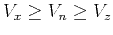 .
Those inequalities follow from the definitions of , ,
, and the Cauchy-Schwartz inequality. They reduce to equalities only
when velocity is constant. Linearizing expression
(34) with respect to Thomsen's anisotropic parameters
.
Those inequalities follow from the definitions of , ,
, and the Cauchy-Schwartz inequality. They reduce to equalities only
when velocity is constant. Linearizing expression
(34) with respect to Thomsen's anisotropic parameters  and
and  , we can transform it to the form analogous to
that of equation (5):
, we can transform it to the form analogous to
that of equation (5):
![\begin{displaymath}
V_g^2(\psi) = V_z^2 \left[ 1 + 2 \delta \sin^2{\psi} +
2 \eta (1 - \cos{\psi})^2\right]\;.
\end{displaymath}](img96.png) |
(35) |
Figure 3 illustrates the difference between the VTI
model and the effective anisotropy implied by the Malovichko approximation.
The differences are noticeable in both the shapes of the effective wavefronts
(Figure 3a) and the moveouts (Figure 3b).

|
|---|
nmofrz
Figure 3. Comparison of the
wavefronts (a) and moveouts (b) in the VTI (solid) and vertically
inhomogeneous isotropic media (dashed). The values of the effective
vertical, horizontal, and NMO velocities are the same
in both media and correspond to Thomsen's parameters
 and and
 . .
|
|---|
![[png]](icons/viewmag.png) ![[mathematica]](icons/mathematica.png)
|
|---|
In deriving equation (35), we have assumed the correspondence
 |
(36) |
We could also have chosen the value of the parameter of heterogeneity that
matches the coefficient given by equation (25) with
the corresponding term in the Taylor series (13).Then, the value of is (Alkhalifah, 1997)
 |
(37) |
The difference between equations (36) and (37) is an
additional indicator of the fundamental difference between homogeneous
VTI and vertically heterogeneous isotropic media. The three-parameter
anisotropic approximation (12) can match the
reflection moveout in the isotropic model up to
the fourth-order term in the Taylor series expansion if the value of
 is chosen in accordance with equation (37). We can
estimate the error of such an approximation with an equation analogous
to (32):
is chosen in accordance with equation (37). We can
estimate the error of such an approximation with an equation analogous
to (32):
 |
(38) |
The difference between the error estimates (32) and
(38) is
 |
(39) |
For usual values of
, which range from to , the expression (39) is
positive. This means that the anisotropic approximation
(12) overestimates traveltimes in the isotropic
heterogeneous model even more than does the shifted hyperbola
(30) shown in Figure 3b.
Below, we examine which of the two approximations is more suitable when
the model includes both vertical heterogeneity and anisotropy.
|
|
|
|
| Nonhyperbolic reflection moveout of -waves:
An overview and comparison of reasons | |
|
Next: Vertically heterogeneous VTI model
Up: VERTICAL HETEROGENEITY
Previous: VERTICAL HETEROGENEITY
2013-03-03