 |
 |
 |
 | Nonhyperbolic reflection moveout of  -waves:
An overview and comparison of reasons -waves:
An overview and comparison of reasons |  |
![[pdf]](icons/pdf.png) |
Next: VERTICAL HETEROGENEITY
Up: Fomel & Grechka: Nonhyperbolic
Previous: WEAK ANISOTROPY APPROXIMATION for
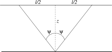
To exemplify the use of weak anisotropy, let us consider the
simplest model of a homogeneous VTI medium above a horizontal
reflector. For an isotropic medium, the reflection traveltime curve is
an exact hyperbola, as follows directly from the Pythagorean theorem
(Figure 2)
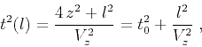 |
(9) |
where  denotes the depth of reflector,
  is the offset,
 is the zero-offset traveltime, and
  is the
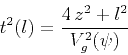
isotropic velocity. For a homogeneous VTI medium, the
velocity in equation (9) is replaced by the
angle-dependent group velocity
is the
isotropic velocity. For a homogeneous VTI medium, the
velocity in equation (9) is replaced by the
angle-dependent group velocity  . This replacement leads to the
exact traveltimes if no approximation for the group velocity is used,
since the ray trajectories in homogeneous VTI media remain straight,
and the reflection point does not move.
We can also obtain an approximate traveltime using the
approximate velocity defined by equations (1) or
(5), where the ray angle
. This replacement leads to the
exact traveltimes if no approximation for the group velocity is used,
since the ray trajectories in homogeneous VTI media remain straight,
and the reflection point does not move.
We can also obtain an approximate traveltime using the
approximate velocity defined by equations (1) or
(5), where the ray angle  is given by
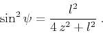 |
(10) |
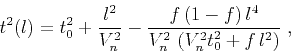
Substituting equation (10) into (5) and
linearizing the expression
 |
(11) |
with respect to the anisotropic parameters  and
and  , we arrive
at the three-parameter nonhyperbolic approximation (Tsvankin and Thomsen, 1994)
, we arrive
at the three-parameter nonhyperbolic approximation (Tsvankin and Thomsen, 1994)
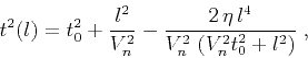 |
(12) |
where the normal-moveout velocity  is defined by equation
(4). At small offsets
is defined by equation
(4). At small offsets  , the influence of the
parameter is negligible, and the traveltime curve is nearly
hyperbolic. At large offsets
, the influence of the
parameter is negligible, and the traveltime curve is nearly
hyperbolic. At large offsets  , the third term in equation
(12) has a clear influence on the traveltime behavior.
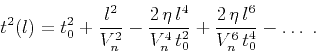
The Taylor series expansion of equation (12) in the vicinity
of the vertical zero-offset ray has the form
, the third term in equation
(12) has a clear influence on the traveltime behavior.
The Taylor series expansion of equation (12) in the vicinity
of the vertical zero-offset ray has the form
 |
(13) |
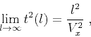
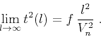
When the offset approaches infinity, the traveltime
approximately satisfies an intuitively reasonable relationship
 |
(14) |
where the horizontal velocity  is defined by equation (3).
Approximation (12) is analogous, within the weak-anisotropy assumption, to the ``skewed hyperbola'' equation
(Byun et al., 1989) which uses the three velocities , ,
and as the parameters of the approximation:
is defined by equation (3).
Approximation (12) is analogous, within the weak-anisotropy assumption, to the ``skewed hyperbola'' equation
(Byun et al., 1989) which uses the three velocities , ,
and as the parameters of the approximation:
 |
(15) |
The accuracy of equation (12), which usually lies within 1% error up to offsets twice as large as reflector depth, can be further improved at any
finite offset by modifying the denominator of the third term
(Grechka and Tsvankin, 1998; Alkhalifah and Tsvankin, 1995).
|
|---|
nmoone
Figure 2. Reflected rays
in a homogeneous VTI layer above a horizontal reflector (a scheme).
|
|---|
![[png]](icons/viewmag.png) ![[xfig]](icons/xfig.png)
|
|---|
Muir and Dellinger (1985) suggested a different nonhyperbolic moveout
approximation in the form
 |
(16) |
where  is the dimensionless parameter of anellipticity. At large
offsets, equation (16) approaches
is the dimensionless parameter of anellipticity. At large
offsets, equation (16) approaches
 |
(17) |
Comparing equations (14) and (17), we
can establish the correspondence
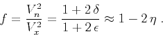 |
(18) |
Taking this equality into account, we see that equation
(16) is approximately equivalent to equation
(12) in the sense that their difference has the order
of  .
.
|
|
|
|
| Nonhyperbolic reflection moveout of -waves:
An overview and comparison of reasons | |
|
Next: VERTICAL HETEROGENEITY
Up: Fomel & Grechka: Nonhyperbolic
Previous: WEAK ANISOTROPY APPROXIMATION for
2013-03-03